Every program is two things bolted together: somewhere to put the data, and a set of steps that does something with it. The first is a data structure. The second is an algorithm. DSA is those two words shortened, and the acronym frightens people considerably more than the subject deserves.
Here is why it is worth your time, in one number. Searching a Python list of a million items for a value sitting at the end inspects a million slots. Asking a Python set the same question inspects about one. Same data, same machine — a million times the work, decided entirely by where the data was put. No faster laptop gets that back. It is a structural choice, and you make it before the first line of code.
So the subject is smaller than it sounds: a handful of ways to arrange data, a handful of standard procedures that run over them, and a way of measuring cost that compares two approaches before you build either. Below: what those words mean, how to judge speed without a stopwatch, how to think when a problem is new to you, where DSA shows up in real systems, and which language to learn it in.
Data structures: where the data sits
A data structure is a layout. It decides which questions are cheap to answer and which are expensive, and every structure trades one for the other.
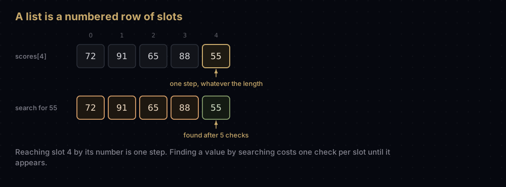
Start with the one you already know. A Python list is a numbered row of slots. The numbering is not decoration. It is the entire reason lists are fast at what they are fast at. The computer knows where the row starts and how wide each slot is, so it reaches slot 4 by doing one multiplication and one addition. It does not walk past slots 0 through 3 to get there.
# A list is a numbered row of slots, and the number is the whole point.
scores = [72, 91, 65, 88, 55]

print(scores[0])
print(scores[4])
print(len(scores))72
55
5Both of those lookups cost the same, whether the list holds five items or five million. That is what "constant time" means in practice.
Now ask a different question: where is the score for Chen? The list does not know. Positions are numbered, not named, so the only honest answer is to look at every name in turn until one matches.
def find_score(names: list[str], scores: list[int], wanted: str) -> tuple[int, int]:
    """Return the wanted student's score and how many names were inspected.

    A score of -1 means the name is not in the list at all.
    """
    for position, name in enumerate(names):
        if name == wanted:
            return scores[position], position + 1
    return -1, len(names)


names = ["Asha", "Ben", "Chen", "Dara", "Esi"]

print(find_score(names, scores, "Asha"))
print(find_score(names, scores, "Esi"))
print(find_score(names, scores, "Farid"))(72, 1)
(55, 5)
(-1, 5)Three results, two different costs. A name at the front is found immediately. A name at the back costs a full sweep, and so does a name that is absent, because you cannot rule it out until you have checked everything. That last case is the one that matters: on a list of n names, the worst case is n inspections.
A dictionary answers the same question differently. You hand it a key, it runs the key through a hash function that turns it into a slot number, and it goes straight to that slot.
by_name = {"Asha": 72, "Ben": 91, "Chen": 65, "Dara": 88, "Esi": 55}

print(by_name["Esi"])
print(by_name.get("Farid", "not enrolled"))55
not enrolled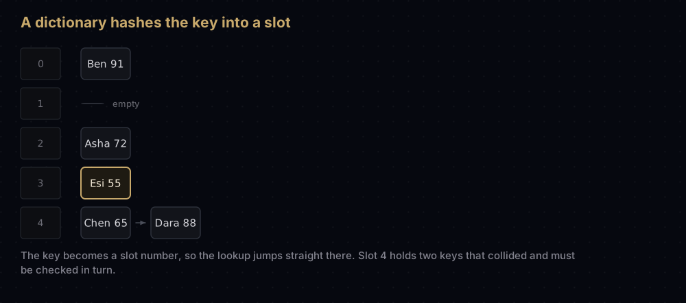
The slot numbers in that diagram are illustrative: Python's real hashes are large integers, reduced to a slot by the table's size. Two different keys can land in the same slot, which is called a collision, and the table has to store both and check them. That is why a dictionary lookup is usually one step rather than always one step. Hash tables covers the mechanics properly.
Scale it up and the gap stops being academic:
big_list = list(range(1_000_000))
big_set = set(big_list)


def scan_steps(haystack: list[int], needle: int) -> int:
    """Count how many slots a left-to-right scan inspects before it finds one."""
    for inspected, item in enumerate(haystack, start=1):
        if item == needle:
            return inspected
    return len(haystack)


print("list scan inspected:", scan_steps(big_list, 999_999), "slots")
print("set membership test:", 999_999 in big_set)list scan inspected: 1000000 slots
set membership test: TrueOne million inspections against roughly one. Both lines are one expression of Python. The difference is not skill or syntax. It is which structure the data was sitting in.
Every structure in this series is a variation on that trade. A linked list gives up fast indexing to gain cheap insertion in the middle. A binary search tree gives up constant-time lookup to keep everything in sorted order. A heap never sorts fully, in exchange for always knowing the smallest item instantly. There is no best structure: only the one that makes your most frequent operation cheap.
Algorithms: what you do with the data
An algorithm is a finite sequence of unambiguous steps that turns an input into an output. Three words in that sentence are doing real work.
Finite — it has to stop. A procedure that loops forever on some input is not an algorithm, it is a bug.
Unambiguous — every step must have exactly one meaning. "Sort the list" is not a step. "If this item is larger than the next one, swap them" is.
Input to output — an algorithm is defined by what it promises, not how it feels. "Given a list of numbers, return them in ascending order" is a specification; bubble sort, merge sort and Timsort are three different algorithms that all satisfy it, at wildly different costs.
You already write algorithms. find_score above is one: it takes a list and a name, and it returns a score in a bounded number of steps. What DSA adds is the second question, not "does it work?" but "what does it cost, and how does that cost grow?"
Big O, without the maths
Timing code with a stopwatch tells you about your laptop. Big O tells you about the algorithm.
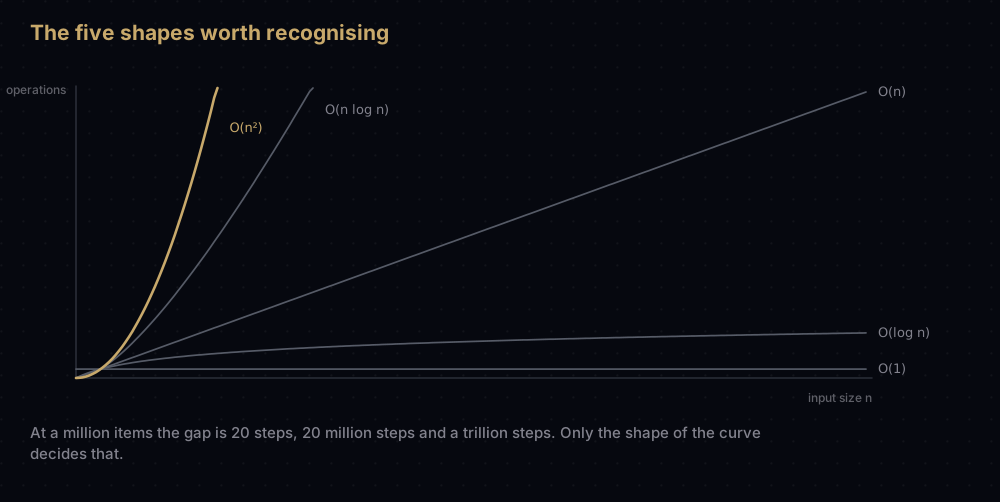
The idea: ignore the constants, ignore the machine, and describe only how the work grows as the input grows. If doubling the input roughly doubles the work, that is O(n). If doubling the input barely changes the work, that is O(1). If doubling the input quadruples the work, that is O(n²).
Five shapes cover almost everything you will meet:
| Shape | Name | Doubling n does what? | Example |
|---|---|---|---|
| O(1) | constant | nothing | scores[4], len(items), a dict lookup |
| O(log n) | logarithmic | adds one step | binary search in a sorted list |
| O(n) | linear | doubles the work | scanning a list, summing it, finding the max |
| O(n log n) | linearithmic | slightly more than doubles | sorted(items), merge sort |
| O(n²) | quadratic | quadruples the work | comparing every pair of items |
The reason O(log n) is so good is worth one sentence, because it recurs constantly. Every step of binary search throws away half of what is left, so the number of steps is the number of times you can halve n before reaching 1, and halving a million takes 20 steps, not 500,000.
Abstract shapes are unconvincing. Real counts are not:
import math

print(f"{'n':>9}  {'log2 n':>6}  {'n log2 n':>12}  {'n squared':>17}")
for n in [10, 100, 1_000, 10_000, 100_000, 1_000_000]:
    log_n = math.log2(n)
print(f"{n:>9,} {log_n:>6.1f} {n * log_n:>12,.0f} {n * n:>17,}") n log2 n n log2 n n squared
10 3.3 33 100
100 6.6 664 10,000
1,000 10.0 9,966 1,000,000
10,000 13.3 132,877 100,000,000
100,000 16.6 1,660,964 10,000,000,000
1,000,000 19.9 19,931,569 1,000,000,000,000Read the last row slowly. At a million items, an O(log n) approach takes about 20 steps and an O(n log n) approach takes about 20 million, but an O(n²) approach takes a trillion. CPython manages on the order of ten million simple operations per second, so the n log n column is a couple of seconds and the n² column is over a day. Same laptop, same problem, different shape.
One honest caveat, because Big O is regularly over-applied: it describes growth, not speed. For 20 items an O(n²) algorithm can easily beat an O(n log n) one, because the constants Big O throws away are real. It is the first question you ask, not the last. The full treatment (the formal definition, best and average and worst case, amortised cost, and how to analyse loops and recursion) is in Big O notation.
How to attack a problem you have never seen
Beginners freeze on unfamiliar problems because they try to produce the clever answer first. Nobody does that. The reliable method has five steps, and the clever answer falls out of step four.
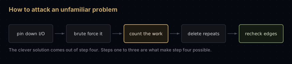
1. Pin down the input and the output. Can the input be empty? Contain duplicates, negatives, one item? What comes back when there is no answer? A large share of failed interviews are someone solving a slightly different problem from the one asked.
2. Solve it by brute force, out loud, on a tiny example. Take five items and do it by hand. If you cannot describe a slow correct method in plain English, no amount of Python will rescue you, and the slow version is what you check the fast one against.
3. Count the work. One loop over n items is n steps. A loop inside a loop is n × n. A step that halves the range is log n. Now you have a number to beat.
4. Find the repeated work and delete it. Almost every optimisation is this. Slow algorithms recompute what they already knew; fast ones remember, in a set, a dictionary, a running total, a cache.
5. Recheck the edges. Empty input, one item, all items identical, the answer at the very first or very last position.
Take a concrete problem: given a list of numbers and a target, do any two of them add up to the target?
The brute force is step two, written down. Try every pair.
def has_pair_bruteforce(numbers: list[int], target: int) -> tuple[bool, int]:
    """Test every pair of positions. Also reports how many pairs were tested."""
    tested = 0
    for left in range(len(numbers)):
        for right in range(left + 1, len(numbers)):
            tested += 1
            if numbers[left] + numbers[right] == target:
                return True, tested
    return False, tested


def has_pair_one_pass(numbers: list[int], target: int) -> tuple[bool, int]:
    """Remember every number seen, so its partner can be looked up directly."""
    seen = set()
    inspected = 0
    for number in numbers:
        inspected += 1
        if target - number in seen:
            return True, inspected
        seen.add(number)
    return False, inspected


values = list(range(1, 2001))

print(has_pair_bruteforce(values, 4001))
print(has_pair_one_pass(values, 4001))
print(has_pair_one_pass([3, 8, 1, 9], 10))(False, 1999000)
(False, 2000)
(True, 4)Step three, the counting argument: the outer loop runs n times, and for each position left the inner loop tests every position after it. That is (n − 1) + (n − 2) + … + 1 pairs, which sums to n(n − 1) / 2. For the 2,000 numbers above that is 2000 × 1999 / 2 = 1,999,000: exactly what the code counted. Quadratic.
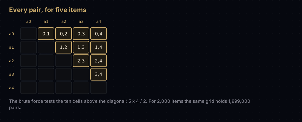
Step four asks what the brute force keeps redoing. By the time the outer loop reaches 900 it has already been paired against every earlier number, and it kept none of that: it starts a fresh forward walk hunting for 3,101. The fix is to remember. Each number's partner is fixed and known: target - number. So keep every number seen so far in a set, and for each new number ask whether its partner is already in there. The set answers in about one step, so the whole thing is one pass: n numbers, one constant-time lookup each, O(n).
That is 2,000 inspections instead of 1,999,000, and the gap widens as n grows. The cost is memory: the set can hold up to n numbers, so you traded O(1) space for O(n) space. That trade — spend memory to save time — is the most common move in the whole subject, and it powers dynamic programming, hash tables and every cache ever written.
The last output line shows it stopping early: on [3, 8, 1, 9] with target 10, 1 was already in the set when 9 arrived, so it returned after 4 inspections.
Which language should you learn DSA in?
Short answer: Python, unless you already know why you need C++.
The reason is that DSA is hard enough on its own, and every line of ceremony between you and the idea is a line where your attention leaks. Compare a swap. In Python it is a, b = b, a. In C++ it is std::swap(a, b), once you have decided whether a is an index or a std::vector<int>::iterator. In Java it is three lines and a temporary variable, inside a class, inside a public static void main. The algorithm is identical; only one version is the algorithm and nothing else.
Python also ships the structures you are learning, which makes it an unusually good study tool. collections.deque is a real double-ended queue, heapq is a real binary heap, bisect is a real binary search, and functools.lru_cache is a real memoiser. Write a structure from scratch to understand it, then check yours against a battle-tested one in the same file. The equivalents exist elsewhere (std::priority_queue and std::lower_bound in C++, PriorityQueue and Collections.binarySearch in Java), but not all one import away.
Now the honest part, because the case for Python is not unconditional.
Competitive programming runs on C++. On Codeforces, ICPC and most contest judges the time limits are calibrated for compiled code, and CPython is commonly 10 to 100 times slower on tight numeric loops. A correct O(n log n) Python solution can time out where the identical C++ solution passes comfortably. If contests are your goal, learn the ideas wherever they are clearest and write your contest code in C++.
Java is still the default in a lot of universities and enterprises. If your course grades Java or your team writes Java, learn DSA in Java: the concepts transfer completely and you avoid a translation step.
Python has two weaknesses worth knowing. Recursion is capped near 1,000 frames by default, so a deep recursive solution raises RecursionError unless you raise the limit or rewrite it as a loop. And the interpreter's constant factor is large, which is why the standard library's heavy lifting is written in C: sorted() runs Timsort in C and beats any sort you write in Python by orders of magnitude.
None of that changes the core point: an algorithm is a way of thinking, not a syntax. Merge sort is merge sort in Python, C++, Java, Go and Rust; only the punctuation moves. Learn it once in the language that gets out of the way, and port it when you need to. This series uses Python for exactly that reason, and if you need the language itself first, start with the complete Python guide.
Where DSA actually shows up
Two places, and the second one is the one people forget.
Interviews. Most large software companies still run a 45-minute problem-solving round: a question you have not seen, a shared editor, and someone watching you think. They are not checking whether you memorised quick sort. They are checking whether you can clarify a problem, produce something correct, notice why it is slow, and improve it: precisely the five-step loop above.
Real systems, constantly. A few you can verify yourself:
- Python's
sorted()andlist.sort()run Timsort, a hybrid of merge sort and insertion sort designed for data that is partly ordered already. - Relational databases index with B-trees — PostgreSQL and MySQL's InnoDB both default to them — because a B-tree keeps lookups logarithmic while matching how disks read in blocks.
- Git stores commit history as a directed acyclic graph, and traversing that graph is what
git logandgit merge-basedo. diffandgit diffwork out how two files differ by finding their longest common subsequence.- Build tools and package managers order work with a topological sort of the dependency graph. That is also how they detect a circular dependency.
- Route planners and game pathfinding use shortest-path algorithms, typically Dijkstra's or A*.
- Redis evicts keys with an approximation of least-recently-used, the same idea as an LRU cache.
You will not implement most of these at work. You will decide, several times a week, whether to scan a list or build a dictionary, and that is the same decision at a smaller scale.
How to learn it, in an order that works
Do not start at "graphs" because a job posting mentioned graphs. The dependencies are real: you cannot understand a hash table without arrays, and you cannot understand a heap without trees.
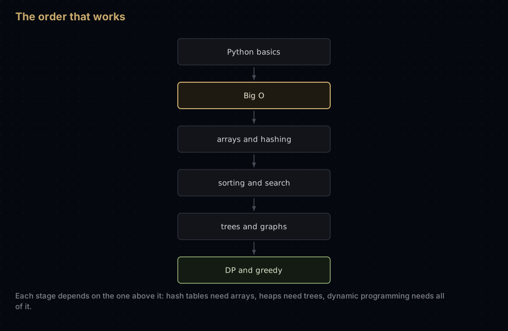
Language basics come first — loops, lists, dictionaries, functions. Then Big O, because every later post assumes you can count work. Then arrays and hashing, the two structures you reach for most days. Then sorting and searching, where you first meet divide and conquer. Then trees and graphs, which are the same idea with more shapes. Then dynamic programming and greedy algorithms, which are strategies rather than structures and are far easier once the rest is solid.
Three habits matter more than the order.
Write the code, do not read the code. Reading a merge sort implementation produces a feeling of understanding that evaporates the moment you face a blank editor. Close the tab and rewrite it from the idea. If you cannot, you have found the gap.
Trace by hand before you run anything. Take five items and step through your loop on paper, writing the variables down after each iteration. Ten minutes of tracing beats an hour of changing signs at random.
Do a small amount, daily, on real problems. Sites like LeetCode, Codeforces and HackerRank exist for this. Two problems a day for three months teaches far more than fourteen on a Saturday, because spacing is what moves a pattern from "I have seen this" to "I recognise this". When you get one wrong, re-derive the answer yourself instead of reading it once and moving on.
What trips beginners up
Memorising solutions. Learning that "two-sum uses a hash map" is worth nothing when the interview asks for three numbers instead of two. Learn why the set removes the repeated work, and the variant solves itself.
Skipping the brute force. Reaching straight for the clever answer usually produces no answer. Write the slow correct version first, always. It is also the reference you test the fast one against.
Confusing the language with the subject. Knowing Python's syntax perfectly is not knowing DSA, and it is the most common way people spend six months and still cannot solve an unfamiliar problem.
Optimising the wrong thing. Shaving a constant factor off an O(n²) loop is pointless when a different structure makes it O(n). Change the shape before you tune the details.
Thinking it is only for interviews. The interview is the exam. Choosing between a list scan and a dictionary lookup in a request handler is the actual subject, and it happens whether or not anyone is watching.
Practice
- Take a list of 20 names, write a loop that returns the position of a given name, and count the inspections for the first name, the last name and an absent name.
- Rewrite that lookup with a dictionary, then say in one sentence what changed about the worst case.
- Find the largest number in a list without using
max(), and state how many comparisons it makes for n items. - Detect whether a list contains a duplicate two ways (comparing every pair, then using a set), and print the work each does on 5,000 distinct items.
- For each of O(1), O(log n), O(n), O(n log n) and O(n²), name one operation you used this week with that cost.
Summary
Data structures decide where data sits; algorithms decide what you do with it; Big O tells you what that combination costs before you build it. Those three ideas are the whole foundation, and the million-to-one gap between scanning a list and querying a set is the clearest evidence that they are worth learning properly.
| Difficulty | Easy |
| Data structure | A layout that makes some operations cheap and others expensive |
| Algorithm | A finite, unambiguous procedure turning an input into an output |
| Why it matters | Structure choice can change cost by a factor of a million; no hardware recovers that |
| First tool to learn | Big O — how work grows with the input, not stopwatch timings |
| Method for a new problem | Pin down I/O, brute force, count the work, delete the repeats, recheck edges |
| Most common optimisation | Spend memory to save time — a set, a dict, a cache |
| Best language to learn in | Python — closest to pseudocode, with heapq / deque / bisect built in |
| Language for contests | C++ — judges assume compiled speed; correct Python can still time out |
| Python's limits | Recursion capped near 1,000 frames; large interpreter constant factor |
| Learning order | Language, Big O, arrays and hashing, sorting and searching, trees and graphs, DP |
| Where it is used | Timsort in sorted(), B-tree indexes, Git's commit DAG, topological sort in build tools |
Start with the language if you need it, then Big O, then the first sort. By the time you have written a sorting algorithm and counted its comparisons yourself, the rest of this series stops feeling like new material and starts feeling like variations on things you already understand.
Keep reading
- Python From Zero — the whole language, from your first variable to classes, if you need it before the algorithms.
- Big O Notation — the rigorous version of the cost argument sketched above, with counting rules for loops and recursion.
- Bubble Sort — the easiest possible first algorithm, and the cheapest place to see an O(n²) counting argument in full.
- Binary Search — where O(log n) comes from, and the clearest payoff for keeping data sorted.
- The Complete Series — all 52 posts, grouped by family, in reading order.


