
Looking a key up in a Python dictionary takes about the same time whether the dictionary holds ten items or ten million. That is not a clever optimisation on top of searching. It is a refusal to search at all: Python computes where the key must be and reads that one place.
The mechanism is a hash table, and the core trick fits in a sentence. Turn the key into a number, and use that number as an array index. Everything else (collisions, load factors, resizing, why a list cannot be a dictionary key) falls out of the problems that one sentence creates.
Sets are hash tables too, and so is the storage behind every attribute you read off an object. Knowing how the table works is what tells you why a lookup is O(1) on average but O(n) in the worst case, and what you have to do to stay on the good side of that line.
The idea
An array gives you one thing for free: values[7] is instant. The machine multiplies 7 by the size of an item, adds that to the start address, and reads. There is no scanning, and the cost does not grow with the length of the array.
Keys are not indices. "banana" is not a position. So you need two steps:
- Hash the key. A hash function reads the key and produces an integer, usually a large one.
- Fold it into range.
hash_value % capacitymaps any integer onto0 .. capacity - 1.
Neither step looks at any other key, so neither one slows down as the table fills. Be precise about what that does not say: hashing reads the whole key — the function below touches every character — so it costs time proportional to the key's length. That length has nothing to do with how many keys you have stored, which is the sense in which the two steps are constant. The slots the result points at are called buckets.
Here is a small hash function you can follow by eye. Python's built-in hash() is randomised per process, so its numbers would not match the ones printed here; this stand-in is deterministic.
def poly_hash(key: str) -> int:
    """Fold every character of a string into one 32-bit integer.

    Multiplying the running total by 31 before adding the next character is
    what makes position matter, so "listen" and "silent" come out different.
    Python's own hash() is randomised per process; this stand-in keeps every
    number in this post reproducible on your machine.
    """
    total = 0
    for character in key:
        total = (total * 31 + ord(character)) & 0xFFFFFFFF
    return total


for key in ["apple", "banana", "cherry", "date", "grape", "lemon"]:
    digest = poly_hash(key)
print(f"{key:<7} hash = {digest:>10} hash % 8 = {digest % 8}")apple hash = 93029210 hash % 8 = 2
banana hash = 2898612069 hash % 8 = 5
cherry hash = 2933454233 hash % 8 = 1
date hash = 3076014 hash % 8 = 6
grape hash = 98615627 hash % 8 = 3
lemon hash = 102857459 hash % 8 = 3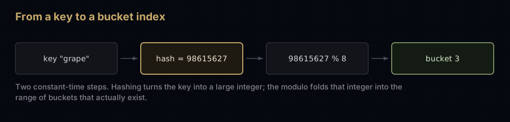
Storing "grape" and finding "grape" run the same two steps and land on the same bucket. That is the whole reason a hash table is fast: lookup is not a search, it is a recomputation.
Collisions are guaranteed
Look at the last two lines. "grape" and "lemon" both land in bucket 3.
That is not bad luck, and a better hash function would not fix it. There are infinitely many possible strings and only 8 buckets, so some must share. Collisions also arrive earlier than intuition suggests. This is the birthday problem, where 23 keys thrown into 365 buckets already collide more often than not. So a hash table is not a hash function plus an array. It is a hash function, an array, and a plan for when two keys want the same slot.
What makes a hash function good
Four properties, in order of how much trouble you get into without them:
- Equal keys must produce equal hashes. A correctness requirement. If
a == bbuthash(a) != hash(b), the two land in different buckets and the table stores both, so you get two entries that compare equal. Nothing else in the design can save you. - Different keys should spread out. The performance requirement. A hash that piles keys into a few buckets turns every lookup into a linear scan.
- It must be cheap. You pay it on every insert, lookup and resize.
- A small change to the input should change the output a lot. Real keys are not random; they are
"user-1","user-2","user-3".
The obvious first attempt fails the second and fourth:
def sum_hash(key: str) -> int:
    """A tempting but poor hash: add up the character codes."""
    return sum(ord(character) for character in key)


print(sum_hash("listen"), sum_hash("silent"), sum_hash("enlist"))
print(poly_hash("listen") % 1024, poly_hash("silent") % 1024, poly_hash("enlist") % 1024)
print("six-letter lowercase words span", sum_hash("aaaaaa"), "to", sum_hash("zzzzzz"))655 655 655
455 85 199
six-letter lowercase words span 582 to 732Adding character codes throws away order, so every anagram collides. Worse, the output barely varies: every six-letter lowercase word hashes to something between 582 and 732, which is 151 distinct values. Give that hash a table of 1,024 buckets and 873 of them stay empty forever. Multiplying by 31 at each step fixes both problems, because each character is scaled by a different power of 31 before it is added in.
Two plans for collisions
Separate chaining. Each bucket holds a small collection — a list — of every pair that landed there. A lookup finds the bucket, then scans it.
Open addressing. Each bucket holds at most one pair. On a collision the insert probes a deterministic sequence of other buckets until it finds a free one, and a lookup walks the same sequence until it finds the key or an empty slot.
Chaining is easier to implement correctly, so that is what gets built below. Open addressing is what CPython's dict uses, and it gets its own section.
Watching it work
Take six keys and eight buckets, using poly_hash and the indices printed above.
def build_table(keys: list[str], capacity: int) -> list[list[str]]:
    """Put each key in bucket poly_hash(key) % capacity, keeping collisions."""
    buckets: list[list[str]] = [[] for _ in range(capacity)]
    for key in keys:
        buckets[poly_hash(key) % capacity].append(key)
    return buckets


def show_table(buckets: list[list[str]]) -> None:
    for index, bucket in enumerate(buckets):
        print(f"  {index:>2} | {' -> '.join(bucket) if bucket else '-'}")


stock_keys = ["apple", "banana", "cherry", "date", "grape", "lemon"]
print(f"capacity 8, {len(stock_keys)} keys, load factor {len(stock_keys) / 8}")
show_table(build_table(stock_keys, 8))

grown = stock_keys + ["fig"]
print(f"capacity 16, {len(grown)} keys, load factor {len(grown) / 16}")
show_table(build_table(grown, 16))capacity 8, 6 keys, load factor 0.75
0 | -
1 | cherry
2 | apple
3 | grape -> lemon
4 | -
5 | banana
6 | date
7 | -
capacity 16, 7 keys, load factor 0.4375
0 | -
1 | -
2 | -
3 | lemon
4 | fig
5 | banana
6 | -
7 | -
8 | -
9 | cherry
10 | apple
11 | grape
12 | -
13 | -
14 | date
15 | -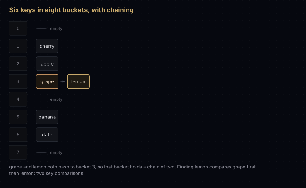
Now trace three operations against the eight-bucket table:
- Find
"lemon". Hash it: 102857459. Fold it:102857459 % 8is 3. Bucket 3 holdsgrapethenlemon, so compare"grape"with"lemon"— not equal — then compare"lemon"with"lemon"— equal. Two key comparisons. - Find
"apple". Bucket 2 holds one entry, which matches. One key comparison. - Find
"kiwi".poly_hash("kiwi")is 3292336, and3292336 % 8is 0. Bucket 0 is empty, so the answer is "not here" after zero key comparisons. A miss on an empty bucket is the cheapest operation a hash table performs.
Notice what decides the cost: not the number of keys in the table, but the number of keys in that one bucket.
Growing the table
Six keys in eight buckets is a load factor of 6 ÷ 8 = 0.75: the average bucket holds 0.75 keys. Add a seventh key and the load factor goes to 0.875, chains start to lengthen, and lookups start to drift away from constant time.
The fix is to grow. Allocate a bigger array of buckets and place every existing key again. You cannot copy buckets across, because the bucket index depends on the capacity: a key in bucket 3 of 8 is not necessarily in bucket 3 of 16.
That is exactly what the second half of the output shows. Adding "fig" triggers a doubling to 16 buckets, and every key is rehashed into the new table.
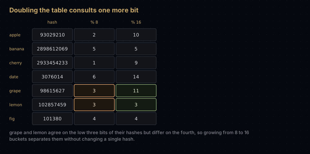
The collision disappears, and the reason is worth seeing. Capacity 8 means the index is the low three bits of the hash, and "grape" and "lemon" happen to agree on those three bits. Capacity 16 means the low four bits decide, and there they differ: 98615627 % 16 is 11, 102857459 % 16 is 3. Doubling the table does not just spread keys out, it consults one more bit of every hash.
The code
Here is the full structure: chaining for collisions, doubling when the load factor passes 0.75.
_MISSING = object()


class HashMap:
    """A hash table with separate chaining and load-factor resizing.

    Each bucket is a list of (key, value) pairs, so several keys can share one
    bucket. Correctness never depends on the hash being good, only on it being
    consistent: equal keys must hash equal. Speed is what depends on the hash
    spreading keys evenly, and on the table growing before chains get long.
    """

    MAX_LOAD = 0.75

    def __init__(self, capacity: int = 8) -> None:
        self._buckets: list[list[tuple[object, object]]] = [[] for _ in range(capacity)]
        self._count = 0

    def _bucket(self, key: object) -> list[tuple[object, object]]:
        # hash() is free to return a negative number. Python's % with a
        # positive modulus always yields a non-negative result, so this index
        # is always in range; in C you would need an explicit mask here.
        return self._buckets[hash(key) % len(self._buckets)]

    def put(self, key: object, value: object) -> None:
        bucket = self._bucket(key)
        for position, (stored_key, _) in enumerate(bucket):
            if stored_key == key:
                bucket[position] = (key, value)  # same key: replace, never append
                return

        bucket.append((key, value))
        self._count += 1
        if self._count > len(self._buckets) * self.MAX_LOAD:
            self._resize(len(self._buckets) * 2)

    def get(self, key: object, default: object = None) -> object:
        for stored_key, value in self._bucket(key):
            if stored_key == key:
                return value
        return default

    def pop(self, key: object, default: object = _MISSING) -> object:
        bucket = self._bucket(key)
        for position, (stored_key, value) in enumerate(bucket):
            if stored_key == key:
                del bucket[position]
                self._count -= 1
                return value
        if default is _MISSING:
            raise KeyError(key)
        return default

    def _resize(self, new_capacity: int) -> None:
        # Every key has to be placed again: the index depends on the capacity,
        # so a key in bucket 3 of 8 is not necessarily in bucket 3 of 16.
        old_buckets = self._buckets
        self._buckets = [[] for _ in range(new_capacity)]
        for bucket in old_buckets:
            for key, value in bucket:
                self._buckets[hash(key) % new_capacity].append((key, value))

    def __contains__(self, key: object) -> bool:
        return any(stored_key == key for stored_key, _ in self._bucket(key))

    def __len__(self) -> int:
        return self._count

    @property
    def capacity(self) -> int:
        return len(self._buckets)

    @property
    def load_factor(self) -> float:
        return self._count / len(self._buckets)
This one uses Python's real hash(), so it accepts any hashable key, not just strings.
stock = HashMap()
for name, count in [("apple", 12), ("banana", 7), ("cherry", 45),
                    ("date", 8), ("grape", 30), ("lemon", 5)]:
    stock.put(name, count)
print(f"{len(stock)} keys, capacity {stock.capacity}, load {stock.load_factor}")

stock.put("fig", 3)  # the seventh key pushes the load factor past 0.75
print(f"{len(stock)} keys, capacity {stock.capacity}, load {stock.load_factor}")

stock.put("apple", 20)  # an existing key: the value is replaced, not appended
print(f"apple = {stock.get('apple')}, keys = {len(stock)}")
print(f"kiwi = {stock.get('kiwi', 0)}, 'kiwi' in stock = {'kiwi' in stock}")
print(f"pop('date') = {stock.pop('date')}, keys = {len(stock)}")

big = HashMap()
for number in range(1000):
    big.put(f"key-{number}", number)
print(f"{len(big)} keys, capacity {big.capacity}, load {big.load_factor:.3f}")6 keys, capacity 8, load 0.75
7 keys, capacity 16, load 0.4375
apple = 20, keys = 7
kiwi = 0, 'kiwi' in stock = False
pop('date') = 8, keys = 6
1000 keys, capacity 2048, load 0.488A thousand keys ended up in 2,048 buckets: the table doubled eight times, from 8 to 2,048, and never let the load factor exceed 0.75.
How the code maps to the idea
_bucket is the whole idea in one line. Hash, fold into range, return the list that lives there. Every other method calls it and then works on a short list. Note the negative-hash detail: hash() may return a negative integer (hash(-1) is -2), and Python's % with a positive modulus always returns a non-negative result, so no extra guard is needed. In C or Java you mask the sign bit off yourself.
put searches its bucket before it appends. Without that loop, put("apple", 20) on an existing key would append a second ("apple", 20) pair, get would keep returning the first one, and len would be wrong forever. Replacing rather than appending is what makes this a hash map rather than a multimap. It also means the resize check only fires when the count really grew.
_resize rehashes rather than copies. It walks every pair in every old bucket and computes a fresh index against the new capacity. This is the one genuinely expensive operation in the structure.
pop raises KeyError unless you pass a default, mirroring dict.pop. The sentinel _MISSING exists because None is a legitimate default value: pop(key, None) must return None quietly rather than raise.
get compares with ==, not is. Two different string objects with the same characters are equal, and a hash table must find a key by value. Real implementations add two shortcuts ahead of that comparison: check identity first, since a hit is almost always the same object, and compare the stored hash values first, since unequal hashes mean unequal keys and comparing two integers beats comparing two long strings. CPython also caches a string's hash inside the string object, so hashing the same string twice costs nothing the second time.
Edge cases fall out for free. An empty bucket makes every loop body run zero times. A missing key falls through to the default. Two unequal keys sharing a bucket are separated by the == check, never by the hash.
Complexity
Count the work in a lookup. One call to hash, one modulo, one list index: none of them depend on how many keys the table holds. Every bound below counts key operations: hashing one key is one unit, comparing two keys is one unit. That convention hides a real cost — hashing a 10,000-character string reads 10,000 characters — but the cost it hides is the same at ten keys and at ten million, and n is the variable these bounds are about. Then a scan of one bucket. So the entire question is: how long is that bucket?
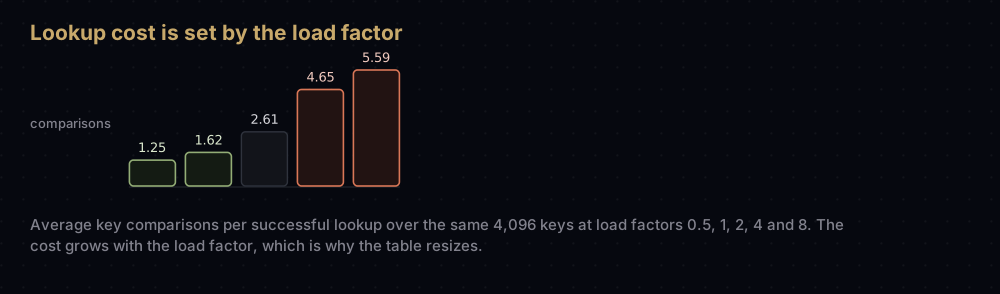
With n keys spread over m buckets, the average bucket holds n / m keys. That ratio is the load factor. If the hash spreads keys uniformly, a successful lookup compares about 1 + load / 2 keys on average, because it stops halfway through the chain it lands in. An unsuccessful lookup scans a whole chain, about load comparisons.
That is a claim you can measure:
def fnv1a(key: str) -> int:
    """FNV-1a, 64 bit: xor each byte in, then multiply by a large odd prime."""
    total = 0xCBF29CE484222325
    for byte in key.encode():
        total = ((total ^ byte) * 0x100000001B3) & 0xFFFFFFFFFFFFFFFF
    return total


def average_lookup_cost(hash_fn, keys: list[str], capacity: int) -> float:
    """Mean number of key comparisons one successful lookup needs."""
    chain_length = [0] * capacity
    comparisons = 0
    for key in keys:
        index = hash_fn(key) % capacity
        chain_length[index] += 1
        comparisons += chain_length[index]  # a new key joins the end of its chain
    return comparisons / len(keys)


sample = [f"user-{number}" for number in range(4096)]
print("load   1 + load/2   poly_hash   fnv1a")
for capacity in [8192, 4096, 2048, 1024, 512]:
    load = len(sample) / capacity
    print(f"{load:>4.1f}   {1 + load / 2:>9.2f}   "
          f"{average_lookup_cost(poly_hash, sample, capacity):>9.2f}   "
f"{average_lookup_cost(fnv1a, sample, capacity):>5.2f}")load 1 + load/2 poly_hash fnv1a
0.5 1.25 1.25 1.18
1.0 1.50 1.62 1.41
2.0 2.00 2.61 1.88
4.0 3.00 4.65 2.84
8.0 5.00 5.59 4.87Three things in that table. The cost tracks the load factor and nothing else: the same 4,096 keys cost 1.25 comparisons at load 0.5 and 5.59 at load 8. FNV-1a sits on or just under the prediction, because it mixes well and these keys are sequential. And poly_hash drifts above it as the table fills, which is what a mediocre hash looks like from the outside: not wrong, just clumpier than random.
Average case: O(1) for lookup, insert and delete. Resizing holds the load factor at or below 0.75 no matter how many keys arrive, so the expected chain length is a constant, so the expected number of comparisons is a constant. The bound is not "small n": it holds at ten keys and at ten million, because the table grew in between.
Insert is O(1) amortised, not worst case. A single insert that triggers a resize does Θ(n) work, because it rehashes every key. But look at when that happens. A table that has just doubled to capacity m holds about 0.375m keys and will not resize again until it holds 0.75m, so at least 0.375m insertions separate one resize from the next. Spread the Θ(m) rehash over those Θ(m) insertions and each carries O(1) extra. That is the same doubling argument that makes list.append amortised O(1): the expensive step gets rarer at exactly the rate it gets more expensive.
Worst case: O(n). If every key lands in the same bucket, that bucket is a list of n entries and a lookup scans all of them. That happens when the hash is bad (return 0 is a legal __hash__), when the keys are pathological for that hash, or when an attacker chose them deliberately. It is why "hash table" and "guaranteed O(1)" are not the same sentence.
Space: O(n). You store n key-value pairs plus a bucket array of m slots, and growth keeps m within a constant factor of n while keys are arriving. A hash table is meaningfully heavier per item than a list: there are empty buckets by design, and a low load factor buys speed with memory. Note what the code never does, though: shrink. Delete all but one of a million keys and the million-slot array is still there, so the honest bound is O(peak n). CPython's dict is the same: deleting keys never hands the memory back.
| Operation | Average | Worst case |
|---|---|---|
| Look up a key | O(1) | O(n) |
| Insert | O(1) amortised | O(n) |
| Delete | O(1) | O(n) |
| Iterate every key | O(n + m) | O(n + m) |
| Find the smallest key | O(n + m) | O(n + m) |
That last row is the honest limitation. A hash table scatters keys by design, so anything involving order (minimum, maximum, "all keys between 10 and 20", sorted output) costs a full scan.
What CPython's dict actually does
The HashMap above is a teaching structure. CPython's dict differs in three ways worth knowing, because each explains behaviour you can observe.
It uses open addressing, not chaining. Each slot holds at most one entry. The probe sequence is not "try the next slot": that clusters badly, because a run of filled slots grows from both ends. CPython mixes the unused high bits of the hash in instead: it keeps a perturb value starting at the full hash, and computes each next slot as 5 * slot + 1 + perturb before shifting perturb right by 5 bits. The early probes therefore depend on the whole hash, not just the low bits that chose the first slot, and once perturb reaches zero the recurrence still reaches every slot in the table.
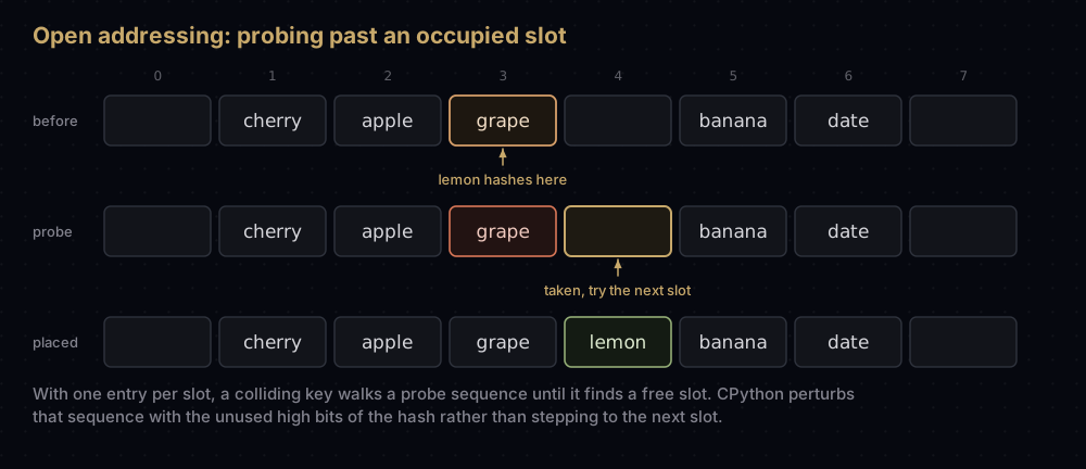
Deletion needs one extra trick. You cannot simply blank a slot, because a lookup probing past it would stop early and miss a key stored further along the sequence. Deleted slots get a tombstone instead (occupied for the purpose of probing, free for the purpose of inserting) cleared out at the next resize.
It is compact, and that is why it keeps insertion order. Since Python 3.6 a dict is two arrays: a sparse array of small integers playing the role of the bucket array, and a dense array of (hash, key, value) entries appended in insertion order, with the sparse array storing indices into the dense one. That saves memory, because the sparse part holds one- or two-byte integers for small dicts rather than full pointers. It also makes iteration walk the dense array, which is why dict iterates in insertion order. That ordering was an implementation detail in 3.6 and became a language guarantee in 3.7, so you can rely on it. set uses the same hash machinery but not the compact layout, so sets are not ordered.
It grows at two-thirds full rather than the 0.75 used above, and always to a power of two, so the modulo is a bitwise and.
Hash randomisation, and the attack it stops
Run python3 -c "print(hash('abc'))" twice and you get two different numbers. Since Python 3.3, the hash of a str or bytes mixes in a random seed chosen when the process starts.
The reason is a denial-of-service attack disclosed in 2011 that hit Python, PHP, Java and Ruby alike. When hash("abc") was a fixed, published function, an attacker could pre-compute thousands of distinct strings that all land in the same bucket and send them as form fields in one POST request. Building the dictionary of parameters then hit the worst case: every insert walked a run of colliding entries that was already long, turning O(n) parsing into O(n²) and burning a core on a single request. A per-process seed means the attacker cannot know which strings collide in your process.
Two practical consequences:
PYTHONHASHSEED=0disables randomisation andPYTHONHASHSEED=some_integerfixes it. Use that to reproduce a test failure, never in production.- Never persist a
hash()value or shard data by it. It is not stable across runs. For a stable digest usehashliborzlib.crc32, which are specified and unchanging.
Integers are not randomised, incidentally: hash(n) is n for small non-negative integers.
What can be a key
A key must be hashable: it must have a __hash__ and its hash must never change while it is in the table.
print(hash(1), hash(1.0), hash(True))
print(hash(-1), hash(-2))

lookup = {1: "int"}
lookup[1.0] = "float"
lookup[True] = "bool"
print(lookup, len(lookup))

try:
    hash(["a", "b"])
except TypeError as error:
    print("hashing a list raises", type(error).__name__)

print(hash(("a", "b")) == hash(("a", "b")))1 1 1
-2 -2
{1: 'bool'} 1
hashing a list raises TypeError
TrueTwo things there surprise people. 1, 1.0 and True are equal to each other and hash the same, so they are one key: the value gets replaced twice and the original key object is kept. And lists are unhashable on purpose: a list can change after you insert it, which would strand the entry in a bucket that no longer matches. Tuples of hashable things are hashable, which is why a tuple is the standard composite key.
For your own classes, __hash__ and __eq__ are a pair and must agree.
from dataclasses import dataclass


class Colour:
    """Equal by value, but with no __hash__ of its own."""

    def __init__(self, red: int, green: int, blue: int) -> None:
        self.red, self.green, self.blue = red, green, blue

    def __eq__(self, other: object) -> bool:
        return (isinstance(other, Colour) and (self.red, self.green, self.blue)
                == (other.red, other.green, other.blue))


try:
    {Colour(255, 0, 0): "red"}
except TypeError as error:
    print("Colour:", error)


@dataclass(frozen=True)
class FrozenColour:
    red: int
    green: int
    blue: int


palette = {FrozenColour(255, 0, 0): "red"}
palette[FrozenColour(255, 0, 0)] = "still red"  # an equal key, so it replaces
print(len(palette), palette[FrozenColour(255, 0, 0)])Colour: unhashable type: 'Colour'
1 still redDefining __eq__ without __hash__ sets __hash__ to None, making instances unhashable. Python does this on purpose: the inherited identity-based hash would disagree with your value-based equality, and equal-but-differently-hashed keys are the one failure a hash table cannot recover from. @dataclass(frozen=True) generates both, consistently, which is the answer you want most of the time.
The other half of the contract is that a key's hash must not change while it is stored:
class Version:
    """A key whose hash changes when you mutate it. Never ship this."""

    def __init__(self, number: int) -> None:
        self.number = number

    def __hash__(self) -> int:
        return hash(self.number)

    def __eq__(self, other: object) -> bool:
        return isinstance(other, Version) and self.number == other.number


key = Version(3)
releases = {key: "stable"}
key.number = 9  # the key's hash just changed, but the slot it sits in did not
print(f"key in releases: {key in releases}")
print(f"Version(9) in releases: {Version(9) in releases}")
print(f"len = {len(releases)}, values = {list(releases.values())}")key in releases: False
Version(9) in releases: False
len = 1, values = ['stable']The entry is still there — len says 1 and you can still iterate to it — but no key can reach it. The dictionary looks in the slot for hash(9); the entry is sitting in the slot for hash(3). This is why "hashable" in practice means "immutable": not a language rule, but the only safe way to guarantee the hash stays put.
Finally, the ordering guarantee, which is easy to state precisely:
menu = {"tea": 3, "coffee": 4, "juice": 5}
del menu["coffee"]
menu["coffee"] = 6  # deleted then re-added, so it goes to the end
menu["tea"] = 7     # updated in place, so it keeps its original position
print(list(menu))['tea', 'juice', 'coffee']Updating an existing key keeps its position. Deleting and re-adding moves it to the end. That is insertion order, not "order of last write".
When to use it, and when not to
Use a hash table whenever you look things up by an exact key: an index from ID to record, membership tests, counting occurrences, de-duplication, caching, grouping rows, joining two datasets on a shared field. If you catch yourself writing a loop that scans a list looking for a match, and that loop runs more than once, you want a dict or a set.
The single most common real speedup in Python code is exactly this. Testing value in some_list is O(n) — it compares element by element. Testing value in some_set is O(1). Building the set costs one pass; after that, every check is free by comparison.
Do not reach for a hash table when:
- You need order or range queries. "The five cheapest items", "everything between two dates", "the next key after this one": all O(n) here. Use a sorted list with the
bisectmodule for a mostly-read dataset, or a binary search tree when it changes often; both give O(log n) ordered access. - You need prefix matching. "Every word starting with
car" is not a hash-table question. That is a trie. - You repeatedly need the smallest or largest item. A heap does that in O(log n) per operation; a hash table needs a full scan every time.
- Your keys are already small dense integers. If keys run 0 to 10,000, a plain list indexed directly is faster and much smaller. You already have the index; do not hash it.
- You need worst-case guarantees. A hard-real-time system, or one that accepts attacker-controlled keys and cannot rely on hash randomisation, is better served by a balanced tree at a guaranteed O(log n) than by an average O(1) with an O(n) tail.
Where it shows up in the real world
- Every Python program you have ever run.
dictandsetare hash tables. So is the namespace holding a module's globals, the__dict__behind an object's attributes, and the mapping of keyword arguments at a call site. Attribute access, name lookup andimportall bottom out in hash tables. functools.lru_cacheis a hash table from the argument tuple to the cached result, paired with a circular doubly linked list that tracks recency. That combination is worth studying on its own — see building an LRU cache.collections.Counterandcollections.defaultdictare thin layers overdict, and they are what you should actually reach for when counting or grouping.- Java's
HashMapuses separate chaining, like the code above, with one addition: since Java 8, a bucket that grows past eight entries in a table of at least 64 buckets is converted from a linked list into a red-black tree, which caps the worst case at O(log n) instead of O(n). That is a direct defence against collision attacks. - Redis keeps its entire keyspace in a hash table with chaining, and rehashes incrementally (two tables live at once, with a few buckets migrated on each command), so growing a database of millions of keys never blocks the server for a full rehash.
- Databases use hash tables for hash joins and hash aggregation: build a table on the smaller relation, then stream the larger one past it, which turns an O(n × m) nested loop into O(n + m).
Common mistakes
Mutating a key after inserting it. Covered above: the entry becomes unreachable. If you need a composite key from mutable data, freeze it: a tuple, a frozenset, or a frozen dataclass.
Defining __eq__ without __hash__. Python turns the instance unhashable, and you find out at the first set or dict that touches it. Add __hash__ over the same fields __eq__ uses, or use @dataclass(frozen=True).
Defining __hash__ and __eq__ over different fields. The dangerous version of the previous mistake, because nothing raises. If __eq__ compares three fields and __hash__ uses two, you get keys that compare equal but hash differently, and the table stores both. Always derive the hash from exactly the tuple of fields that equality uses.
Persisting hash() values. Writing hash(name) % shard_count into a database, or into a file read by another process, produces a mapping that changes on the next restart. Use hashlib.sha256 or zlib.crc32 for anything that outlives the process.
Assuming O(1) is a guarantee. It is an average under a decent hash. A custom __hash__ that returns a constant is perfectly legal and makes every operation O(n).
Mutating a dictionary while iterating it. Adding or deleting keys during a for key in mapping loop raises RuntimeError, because a resize would move entries under the iterator. Iterate over list(mapping) if you need to modify as you go.
Using a list where a set belongs. A membership test inside a loop over a list is the classic accidental O(n²). Converting once to a set makes it O(n).
Practice
- Add
keys(),values()anditems()toHashMap, and explain why the order they produce is not the insertion order. - Instrument
getto count key comparisons, then confirm that the average over many lookups matches the1 + load / 2prediction. - Add shrinking: halve the capacity when the load factor drops below 0.15. Explain why halving as soon as it drops below 0.75 would be a bug.
- Replace chaining with open addressing and linear probing, including tombstones for deletion, and check that a delete followed by a lookup of a key further along the probe sequence still succeeds.
- Build the compact layout: a list of
(hash, key, value)entries in insertion order plus an array of indices into it, and show that iteration comes out in insertion order.
Summary
A hash table trades memory and ordering for speed. It computes a bucket from the key instead of searching for it, which makes lookup, insert and delete O(1) on average, but only because the table keeps its load factor low by rehashing everything whenever it fills up, and only as long as the hash function spreads keys well. Get the __hash__ and __eq__ contract wrong, or mutate a key, and the structure does not degrade gracefully; it loses your data in plain sight.
| Difficulty | Medium |
| Average lookup | O(1) — one hash, one modulo, a chain whose expected length is the load factor |
| Average insert | O(1) amortised — a Θ(n) resize is paid for by the Θ(n) inserts before it |
| Average delete | O(1) — find the bucket, remove from the chain |
| Worst case | O(n) — every key collides into one bucket |
| Space | O(n) — entries plus a bucket array proportional to the peak number of keys; it never shrinks |
| Ordered | No key order; CPython's dict does preserve insertion order |
| Range queries | No — a full O(n) scan; use a sorted structure instead |
| Data structure | Array of buckets, plus a hash function and a collision plan |
| Load factor | Resize past 0.75 here; CPython's dict grows at two-thirds full |
| Use it when | Lookup, membership, counting or de-duplication by an exact key |
| Avoid it when | You need sorted order, prefix search, or worst-case guarantees |
| Real-world use | Python dict and set, Java HashMap, the Redis keyspace, database hash joins |
| Python equivalent | dict, set, collections.Counter, collections.defaultdict |
Write the chaining version once, by hand, and the behaviour of every hash table you meet afterwards stops being magic. The interesting follow-up question is what you do when O(1) on average is not good enough, and the answer is always a structure that keeps its keys in order.
Keep reading
- Arrays and Dynamic Arrays — where O(1) indexing comes from, and the same doubling argument applied to
list.append. - Big O Notation — average versus amortised versus worst case, explained properly.
- Binary Search Trees — the ordered alternative, with O(log n) lookups and range queries a hash table cannot do.
- Tries — what to use when the query is a prefix rather than an exact key.
- Building an LRU Cache — a hash table and a linked list combined into the data structure behind every cache.


