Two programmers solve the same problem. One finishes in 0.3 seconds, the other in 0.9 seconds. Which algorithm is better? You cannot tell — not from those numbers, not from any numbers measured that way. The slow one might be on a laptop from 2014, in a virtual machine that was busy, on an input that happened to suit it.
Big O notation answers the question without a stopwatch. Instead of "how long did it take", it asks "how does the cost grow when the input gets bigger". That makes the answer portable: the same on your laptop, on a server, in Python, in Rust, this year and in ten years, because it describes the algorithm rather than the machine.
The notation is the easy part. The valuable part is the counting argument behind it: looking at a loop and saying why it costs what it costs. That is what this builds, from counting operations up to the Master Theorem.
Why a stopwatch is not a measurement
Wall-clock time is a property of one run, not of an algorithm. It changes with the CPU, the language, the memory pressure, whether another process woke up mid-run, and how big the input happened to be.
Worse, it does not extrapolate. You time a function on 1,000 records and it takes 2 milliseconds. How long on 1,000,000 records? The measurement alone cannot tell you. If the function is linear, roughly 2 seconds. If it is O(n log n), about 4 seconds. If it is quadratic, roughly 33 minutes. One measurement, three answers separated by a factor of a thousand.
That is exactly the bug where a feature works fine in testing with 50 rows and falls over in production with 500,000. The timing was real. It just did not measure the thing that mattered.
So measure the growth instead: count the operations performed as a function of input size, and describe how that count behaves as the input heads for infinity. That description is the complexity, and it belongs to the algorithm.
Counting operations instead
Name the input size first. Call it n. For a list, n is the number of items; for a string, the number of characters; for a graph, usually two sizes, V vertices and E edges. For a number being factorised, n is the digit count, not the value: a trap that comes back later.
Now count. The simplest example: adding up a list.
def count_additions(values: list[int]) -> tuple[int, int]:
    """Sum a list, and report how many additions that took."""
    total = 0
    additions = 0
    for value in values:
        total += value
        additions += 1
    return total, additions


for size in (10, 100, 1000, 10000):
    _, additions = count_additions(list(range(size)))
print(f"n = {size:>5} additions = {additions}")n = 10 additions = 10
n = 100 additions = 100
n = 1000 additions = 1000
n = 10000 additions = 10000The count is exactly n. Ten times the input, ten times the work. That is a linear algorithm, written O(n).
Now something that grows differently: checking for a repeated value by comparing every pair.
def has_duplicate_naive(values: list[int]) -> tuple[bool, int]:
    """Look for a repeated value by comparing every unordered pair once."""
    comparisons = 0
    for left in range(len(values)):
        for right in range(left + 1, len(values)):
            comparisons += 1
            if values[left] == values[right]:
                return True, comparisons
    return False, comparisons


for size in (5, 10, 100):
    all_distinct = list(range(size))
    _, comparisons = has_duplicate_naive(all_distinct)
print(f"n = {size:>3} comparisons = {comparisons:>5} n(n-1)/2 = {size * (size - 1) // 2:>5}")n = 5 comparisons = 10 n(n-1)/2 = 10
n = 10 comparisons = 45 n(n-1)/2 = 45
n = 100 comparisons = 4950 n(n-1)/2 = 4950The count is n(n - 1) / 2, which multiplies out to (n² - n) / 2. Ten times the input, roughly a hundred times the work. That is quadratic, O(n²).
Notice what was never specified: how long a comparison takes. It does not matter. Whatever one costs on your machine, the second function does about n² / 2 of them and the first does n, and for large enough n no constant factor can rescue the second.
What O actually means
The informal version — "an upper bound on the growth rate" — is right, and for most work it is enough. The formal definition is short and explains several things that otherwise look arbitrary.
f(n) is O(g(n)) if there exist two positive constants, c and n0, such that f(n) ≤ c · g(n) for every n at or above n0.
Read that as a promise with two escape hatches. The first is c: you may scale g up by any fixed amount. The second is n0: you may ignore all the small inputs. Beyond that point, c · g(n) sits above f(n) forever.
Apply it to the pair-counting function, whose cost is (n² - n) / 2. Choose g(n) = n², c = 1, n0 = 1. Is (n² - n) / 2 ≤ n² for every n at least 1? Comfortably — the left side is never even half the right. So the function is O(n²), formally.
Two consequences fall straight out:
- O is an upper bound, not an exact answer. That same function is also
O(n³)andO(2^n). Both true, both useless, the way "this parcel weighs under a tonne" is true and useless. By convention, saying an algorithm isO(n²)means the tightest bound you know. - O says nothing about small inputs. An
O(n)algorithm may still lose to anO(n²)one on every input you will ever run. The bound only promises what happens eventually.
Omega and Theta
Because O is only an upper bound, two more symbols exist for the other things.
Omega, Ω(g(n)), is the lower bound. f(n) is Ω(g(n)) if f(n) ≥ c · g(n) beyond some n0: it grows at least this fast. Comparison-based sorting is Ω(n log n): no algorithm that sorts by comparing pairs can beat that in the worst case, however clever. That is a statement about the problem, not about one algorithm.
Theta, Θ(g(n)), is both at once. f(n) is Θ(g(n)) when it is both O(g(n)) and Ω(g(n)): tight from above and below. Merge sort is Θ(n log n): it never does better and never does worse.
In conversation and in almost every textbook table, people write O where they mean Θ, and nobody minds. The distinction still matters in a careful proof, and when someone says an algorithm is "at least O(n²)": that sentence is nonsense, and the word they wanted was Omega.
Why constants and lower-order terms are dropped
Suppose you count precisely and get 3n² + 50n + 200 operations. Big O calls that O(n²). Three terms became one and a factor of 3 vanished. That is not laziness.
def cost(n: int) -> int:
    """A made-up but very typical operation count."""
    return 3 * n * n + 50 * n + 200


header = f"{'n':>6}  {'3n^2':>14}  {'50n':>9}  {'200':>5}  {'total':>14}  {'n^2 share':>9}"
print(header)
for n in (1, 10, 100, 1000, 10000):
    quadratic = 3 * n * n
print(f"{n:>6} {quadratic:>14,} {50 * n:>9,} {200:>5} {cost(n):>14,} {quadratic / cost(n):>9.1%}") n 3n^2 50n 200 total n^2 share
1 3 50 200 253 1.2%
10 300 500 200 1,000 30.0%
100 30,000 5,000 200 35,200 85.2%
1000 3,000,000 50,000 200 3,050,200 98.4%
10000 300,000,000 500,000 200 300,500,200 99.8%At n = 1 the quadratic term is 1.2% of the total and the constant 200 dominates. At n = 10,000 it is 99.8% and the other two are rounding error. The 50n term never catches up, because no fixed multiple of n outruns n² forever.
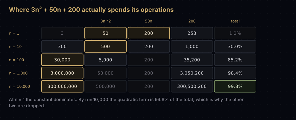
That is the whole justification. Lower-order terms are dropped because the highest-order term eventually accounts for essentially all of the cost. And the constant multiplier is dropped because it does not change the shape of the curve. It is the difference between a fast machine and a slow one, and Big O refuses to care which you own.
When dropping them misleads you
This is the part people skip, then get burned by.
Small inputs live entirely in the discarded terms. At n = 10 above, the 50n term beats the n² term. Real libraries know this: CPython's list sort switches to binary insertion sort, an O(n²) algorithm, for runs shorter than 64 elements, because its constant factor is tiny. An asymptotically worse algorithm wins in the region Big O refuses to describe.
Some constants are enormous. Matrix-multiplication algorithms exist with better exponents than the practical ones and constants so large they would only pay off on matrices bigger than any computer could hold: galactic algorithms, they are called. Closer to home, an O(1) hash lookup still has to hash the key, and hashing a long string costs time proportional to its length; the O(1) is per lookup, not per byte.
The memory hierarchy hides inside the constant. An array and a linked list both traverse in O(n), and the array wins badly in practice because its elements sit next to each other in memory instead of scattered behind pointers.
The bound may be worst case only. Quicksort is O(n²) in the worst case and still beats merge sort in practice almost always. The worst-case letter alone gives you the wrong answer.
The rule to carry: Big O tells you what happens as n grows. To choose between two algorithms at a fixed, known, small n, measure.
The complexity classes you will actually meet
Seven classes cover nearly everything you will meet.
| Class | Name | You get it from |
|---|---|---|
O(1) | constant | values[5], a dict lookup, stack push and pop |
O(log n) | logarithmic | Binary search, balanced-tree insert, fast exponentiation |
O(n) | linear | Summing a list, linear search, one pass over a file |
O(n log n) | linearithmic | Merge sort, heap sort, Python's sorted() |
O(n²) | quadratic | Bubble sort, comparing every pair |
O(2^n) | exponential | Naive recursive Fibonacci, every subset |
O(n!) | factorial | Brute-force travelling salesman, every permutation |
The names are less instructive than the numbers. The operation count each class implies, rounded:
| Class | n = 10 | n = 100 | n = 1,000 | n = 1,000,000 |
|---|---|---|---|---|
O(1) | 1 | 1 | 1 | 1 |
O(log n) | 3 | 7 | 10 | 20 |
O(n) | 10 | 100 | 1,000 | 1,000,000 |
O(n log n) | 33 | 664 | 9,966 | 19,931,569 |
O(n²) | 100 | 10,000 | 1,000,000 | 1,000,000,000,000 |
O(2^n) | 1,024 | 1.3 × 10³⁰ | 1.1 × 10³⁰¹ | unwritable |
O(n!) | 3,628,800 | 9.3 × 10¹⁵⁷ | unwritable | unwritable |
Put a clock on the interesting cells. At a billion operations per second (optimistic for Python, reasonable for C) a million items costs about 20 milliseconds at O(n log n) and about 17 minutes at O(n²). At n = 100, an O(2^n) algorithm needs 1.3 × 10³⁰ operations, roughly 40 thousand billion years; the universe is about 14 billion years old. Exponential algorithms are not "slow", they are impossible, and escaping them is the point of dynamic programming and greedy algorithms.
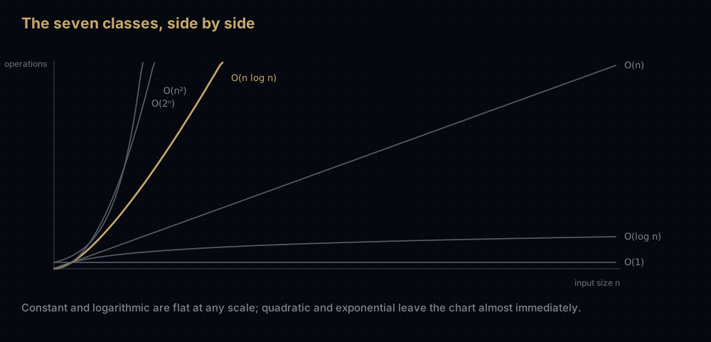
Two rows deserve a note. O(log n) barely grows: doubling the input adds one step, which is why binary search finds an item among a billion in 30 comparisons. And O(n log n) sits close to O(n) at any realistic size — at a million items the log factor is only 20 — which is why "sort it first" is such a cheap move.
Reading complexity off code
Most of the time you do not need a proof. You need four rules.
Sequential statements add
One thing after another costs the sum of the parts, and the sum is dominated by the largest.
Nested loops multiply
A loop inside a loop runs the inner body once for every combination.
A loop over a different input is n times m
Where the most common misreading happens. A nested loop is only O(n²) if both loops range over the same size.
A loop that halves is log n
If each iteration discards a constant fraction of what is left, the iteration count is logarithmic.
All four, counted:
def two_sequential_loops(values: list[int]) -> int:
    """Two loops one after the other. The counts add, they do not multiply."""
    steps = 0
    for _ in values:
        steps += 1
    for _ in values:
        steps += 1
    return steps


def two_nested_loops(values: list[int]) -> int:
    """One loop inside the other over the same input. The counts multiply."""
    steps = 0
    for _ in values:
        for _ in values:
            steps += 1
    return steps


def loops_over_two_inputs(rows: list[int], columns: list[int]) -> int:
    """A nested loop over a different input is n * m, which is not n squared."""
    steps = 0
    for _ in rows:
        for _ in columns:
            steps += 1
    return steps


def halving_loop(n: int) -> int:
    """Each step throws away half of whatever is left."""
    steps = 0
    remaining = n
    while remaining > 1:
        remaining //= 2
        steps += 1
    return steps


data = list(range(1000))
print("sequential loops over n=1000 :", two_sequential_loops(data))
print("nested loops over n=1000     :", two_nested_loops(data))
print("n=1000 rows by m=8 columns   :", loops_over_two_inputs(data, list(range(8))))
print("halvings from 1,000          :", halving_loop(1000))
print("halvings from 1,000,000 :", halving_loop(1_000_000))sequential loops over n=1000 : 2000
nested loops over n=1000 : 1000000
n=1000 rows by m=8 columns : 8000
halvings from 1,000 : 9
halvings from 1,000,000 : 19Each of those four numbers is a rule.
2,000 for the sequential loops. That is 2n, and 2n is O(n). Two passes over a list is not quadratic; it is linear with a constant of 2, and the constant is dropped. Ten passes would still be O(n). Sequential means add. Two loops in a function is not what makes it quadratic. Nesting is.
1,000,000 for the nested loops. That is n × n. Nesting means multiply.
8,000 for the two-input version. That is n × m with n = 1000 and m = 8, and it must be written O(n·m), not O(n²). When m is a small fixed number (the 8 fields of a record, the 26 letters of the alphabet) O(n·m) is O(n) in disguise, because m is a constant. Calling it O(n²) would make you reject a perfectly linear algorithm.
9 halvings from 1,000, and only 19 from 1,000,000. A thousand times the input, barely twice the work. That is log₂(n). The base never appears in the notation: log₂ n and log₁₀ n differ by a constant factor of about 3.32, so every logarithm is O(log n).
The nested case has one refinement, the shape of the duplicate check from earlier. When the inner loop starts at left + 1, it visits only the pairs above the diagonal:
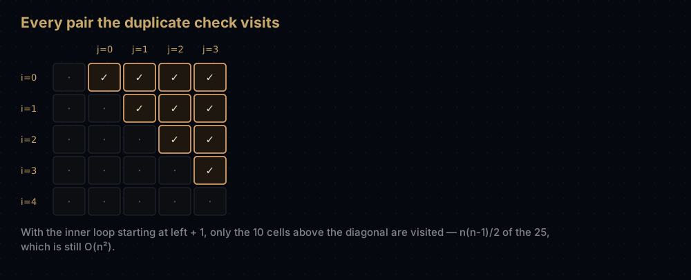
Ten of the 25 cells, which is n(n - 1) / 2. Half the work of the full grid, and still O(n²): halving a quantity does not change how it grows.
One more rule, not about loops at all: a function call costs whatever that function costs. Writing if item in seen_list inside a loop over n items looks like one line, but in on a list is a linear scan, so the loop is O(n²). Make seen_list a set and that line becomes O(1) on average, so the loop becomes O(n). That substitution is probably the highest-value complexity fix in everyday Python.
Best, average and worst case
The same algorithm can cost wildly different amounts on different inputs of the same size. Linear search shows it plainly.
def linear_search(values: list[int], target: int) -> tuple[int, int]:
    """Return the index of target (or -1) plus the comparisons it took."""
    comparisons = 0
    for index, value in enumerate(values):
        comparisons += 1
        if value == target:
            return index, comparisons
    return -1, comparisons


hundred = list(range(100))
for label, target in [("first item", 0), ("middle item", 49),
                      ("last item", 99), ("absent", -1)]:
    index, comparisons = linear_search(hundred, target)
    print(f"{label:<12} index = {index:<4} comparisons = {comparisons}")

average = sum(linear_search(hundred, target)[1] for target in hundred) / len(hundred)
print(f"average over all 100 present targets: {average}")first item index = 0 comparisons = 1
middle item index = 49 comparisons = 50
last item index = 99 comparisons = 100
absent index = -1 comparisons = 100
average over all 100 present targets: 50.5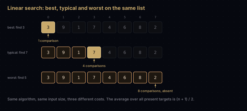
- Best case,
O(1). The target is the first item. One comparison, however long the list is. - Worst case,
O(n). The target is last, or absent. Every element is compared. - Average case,
O(n). Averaged over every position the target could occupy, the count is(n + 1) / 2: 50.5 for a hundred items, exactly as printed. Half ofnis stillO(n).
Average case is the honest default, because it describes the inputs you actually get. Quoting the best case is close to dishonest: every algorithm has a lucky input, and "bogosort is O(n) in the best case" is true and tells you nothing.
Quote the worst case too whenever it differs, and treat it as the number that matters in three situations:
- Latency guarantees. If a request must return in 50 milliseconds, the worst case is the budget.
- Adversarial input. An attacker who picks the input picks the worst case. Hash-collision denial of service is exactly this: feed a server keys that all land in one bucket and
O(1)dictionary inserts becomeO(n), making the requestO(n²). Python has randomised string hashes by default since 3.3 to prevent it. - Recursion depth. A worst case
O(n)deep instead ofO(log n)deep is a stack overflow.
The classic gap is quicksort: Θ(n log n) on average, Θ(n²) when the pivot is always the smallest remaining element. It is still what Java's Arrays.sort uses on primitive arrays and what sits at the core of C++'s std::sort, because that worst case is rare, cheap to avoid, and the average-case constant is excellent.
Space complexity, including the call stack
Space complexity counts the extra memory needed beyond the input itself. The input is not counted: otherwise every algorithm would be O(n) and the measure would say nothing.
- Bubble sort swaps inside the list and needs a handful of variables:
O(1), or in place. - Merge sort builds new lists while merging:
O(n). - Counting sort allocates one slot per distinct key:
O(k)for a key range ofk. - Building a set of every item seen so far:
O(n).
The forgotten part is recursion. Every pending call keeps a stack frame alive (arguments, locals, return address), and those frames are memory even though your code allocates nothing.
import sys

# Pinned so the failure below is a clean RecursionError on every machine.
sys.setrecursionlimit(1500)


def recursive_sum(values: list[int], index: int = 0) -> tuple[int, int]:
    """Sum by recursion, also reporting the deepest stack it needed."""
    if index == len(values):
        return 0, 1
    total, depth = recursive_sum(values, index + 1)
    return values[index] + total, depth + 1


for size in (10, 100, 900):
    total, depth = recursive_sum(list(range(1, size + 1)))
    print(f"n = {size:>3}   total = {total:>6}   peak stack frames = {depth}")

try:
    recursive_sum(list(range(100_000)))
except RecursionError:
print("n = 100000 RecursionError — the call stack is a real space cost")n = 10 total = 55 peak stack frames = 11
n = 100 total = 5050 peak stack frames = 101
n = 900 total = 405450 peak stack frames = 901
n = 100000 RecursionError — the call stack is a real space costThe frame count is n + 1, so this "no extra memory" function is O(n) space, and on 100,000 items it does not run out of time: it runs out of stack. The equivalent loop is O(1) space with no such limit. CPython's default recursion limit is 1,000 for exactly this reason, and raising it is usually the wrong fix.
Depth, not call count, is what you measure. Merge sort makes O(n) recursive calls but only O(log n) are alive at once, so its stack cost is O(log n) and its O(n) space comes from the merge buffers instead. A recursive binary search is O(log n) in both time and stack. A quicksort that recurses into the larger partition first can reach O(n) depth; taking the smaller side first keeps it at O(log n).
Amortised analysis, and why append is O(1)
Some operations are usually cheap and occasionally expensive. Averaging over the whole sequence, rather than quoting the expensive case, is amortised analysis, and the standard example is the dynamic array, which is exactly what a Python list is.
A list stores its elements in one contiguous block of memory. When the block is full and you append again, the implementation allocates a bigger block and copies everything across. That copy is O(n), and if it happened on every append, adding n items would cost O(n²).
The trick is how much bigger the new block is. Grow by a fixed amount — say 10 slots — and you copy every 10 appends, so the total really is quadratic. Double the capacity instead and the expensive copies get exponentially rarer as the list grows.
def append_costs(count: int) -> list[int]:
    """Cost of each append into a doubling array: one unit to write the value,
    plus one unit per element copied when a full block has to be reallocated."""
    costs = []
    capacity = 0
    length = 0
    for _ in range(count):
        cost_here = 1
        if length == capacity:
            capacity = 1 if capacity == 0 else capacity * 2
            cost_here += length  # every stored element is copied to the new block
        costs.append(cost_here)
        length += 1
    return costs


print("cost of each of the first 16 appends:", append_costs(16))
for count in (16, 1024, 1_000_000):
    total = sum(append_costs(count))
print(f"n = {count:>9,} total cost = {total:>10,} per append = {total / count:.2f}")cost of each of the first 16 appends: [1, 2, 3, 1, 5, 1, 1, 1, 9, 1, 1, 1, 1, 1, 1, 1]
n = 16 total cost = 31 per append = 1.94
n = 1,024 total cost = 2,047 per append = 2.00
n = 1,000,000 total cost = 2,048,575 per append = 2.05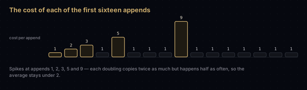
Most appends cost 1. The spikes land at appends 2, 3, 5 and 9 — one past each power of two — and each spike is twice as tall as the last but happens half as often, so the effects cancel.
In closed form: appending n items does n writes plus the copies at each doubling, and those copies total 1 + 2 + 4 + … up to the final capacity, a geometric series summing to one less than that capacity. The final capacity is the first power of two at or above n, so it is under 2n and the whole sequence costs under 3n. That is what the last column measures: 2.00 per append at 1,024 items, 2.05 at a million, bounded by a constant either way. That is O(1) amortised: any single append may cost O(n), but any sequence of n appends costs O(n) overall.
CPython's list uses this strategy (with a growth factor nearer 1.125 than 2, trading extra copies for less wasted memory), which is what makes list.append amortised constant time. Two consequences:
list.pop()from the end isO(1);list.pop(0)from the front isO(n), because every remaining element shifts down one slot. Popping from the front in a loop is a silentO(n²). Usecollections.deque, which isO(1)at both ends.- Amortised is not worst case. A single append can still stall while a million elements are copied. If you need a hard latency bound rather than good throughput, amortised
O(1)is not the guarantee you want.
Recursion, recurrences and the Master Theorem
For a loop you count iterations. For a recursive function you write a recurrence relation: an equation defining the cost at size n in terms of the smaller pieces it calls.
Merge sort splits the list in half, sorts each half recursively, then merges the two sorted halves in one linear pass:
T(n) = 2 · T(n/2) + Θ(n)
T(1) = Θ(1)
Read it literally: two subproblems, each of half the size, plus linear work to combine. Solve it by drawing the recursion tree.
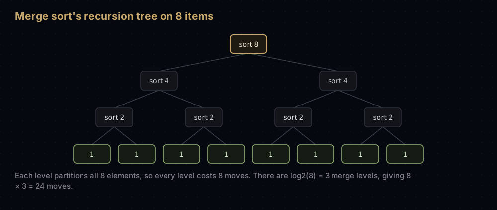
The root merges 8 elements. Its two children merge 4 each: 8 elements of work again. Their four children merge 2 each — 8 again. Every level costs the same n, because the subproblems at a level always partition the whole input. The number of levels is however many times you can halve n before reaching 1, which is log₂ n. Total: n per level times log₂ n levels, so Θ(n log n).
That is not hand-waving. Count the moves:
import math


def merge_sort_counted(values: list[int]) -> tuple[list[int], int]:
    """Merge sort that also reports how many elements the merges moved."""
    if len(values) <= 1:
        return values, 0

    middle = len(values) // 2
    left, left_moves = merge_sort_counted(values[:middle])
    right, right_moves = merge_sort_counted(values[middle:])

    merged: list[int] = []
    left_index = right_index = 0
    while left_index < len(left) and right_index < len(right):
        if left[left_index] <= right[right_index]:
            merged.append(left[left_index])
            left_index += 1
        else:
            merged.append(right[right_index])
            right_index += 1
    merged.extend(left[left_index:])
    merged.extend(right[right_index:])

    # Every element of this subproblem is moved exactly once by the merge.
    return merged, left_moves + right_moves + len(merged)


for size in (8, 64, 1024):
    ordered, moves = merge_sort_counted(list(reversed(range(size))))
    levels = int(math.log2(size))
print(f"n = {size:>4} moves = {moves:>6} n * log2(n) = {size * levels:>6} sorted = {ordered == sorted(ordered)}")n = 8 moves = 24 n * log2(n) = 24 sorted = True
n = 64 moves = 384 n * log2(n) = 384 sorted = True
n = 1024 moves = 10240 n * log2(n) = 10240 sorted = TrueNot approximately n log₂ n. Exactly n log₂ n, for every power of two.
The Master Theorem
Drawing the tree every time gets tedious, so there is a shortcut covering the whole divide-and-conquer family. For a recurrence of the form
T(n) = a · T(n/b) + f(n)where a is at least 1 (how many subproblems), b is greater than 1 (the factor each subproblem shrinks by), and the combining work f(n) is Θ(n^d), compare d against log_b(a):
- If
d < log_b(a), the leaves dominate:T(n) = Θ(n^(log_b a)). So many subproblems that the bottom of the tree accounts for everything. - If
d = log_b(a), every level costs the same:T(n) = Θ(n^d · log n). The extralog nis the number of levels. - If
d > log_b(a), the root dominates:T(n) = Θ(n^d). The top-level combining work swamps everything below it.
The quantity log_b(a) describes how fast the subproblems multiply relative to how fast they shrink. Three worked examples:
Merge sort. T(n) = 2·T(n/2) + Θ(n), so a = 2, b = 2, d = 1. Since log₂(2) = 1, which equals d, this is the middle case: Θ(n¹ · log n) = Θ(n log n). That matches the tree and the measured 10,240 moves for 1,024 items.
Binary search. It discards half the list and recurses into one side, doing constant work to choose: T(n) = 1·T(n/2) + Θ(1), so a = 1, b = 2, d = 0. Since log₂(1) = 0, which equals d, the middle case again: Θ(n⁰ · log n) = Θ(log n). The halving_loop counter measured the same thing: 19 steps for a million items. Python's bisect does this in C.
Karatsuba multiplication. Two n-digit numbers, three recursive half-size multiplications, linear additions: T(n) = 3·T(n/2) + Θ(n), so a = 3, b = 2, d = 1, and log₂(3) ≈ 1.585, greater than d. First case, leaves dominate: Θ(n^1.585). That beats the Θ(n²) schoolbook method, and CPython switches to Karatsuba for large integers.
When the Master Theorem does not apply
It only covers recurrences where every subproblem is the same fraction of the original. Plenty are not:
- Quicksort's worst case is
T(n) = T(n - 1) + Θ(n)— the pivot splits off one element, not a fixed fraction. Expanding givesn + (n-1) + (n-2) + … = Θ(n²). - Naive recursive Fibonacci is
T(n) = T(n - 1) + T(n - 2) + Θ(1), which grows like1.618^n. Memoisation collapses the tree tondistinct subproblems and turns it intoΘ(n). - Unequal splits, like
T(n) = T(n/3) + T(2n/3) + Θ(n), need a tree argument. This one isΘ(n log n)because the longest root-to-leaf path is still logarithmic.
For anything the theorem misses, draw the tree, work out the cost per level, and add the levels up. That method never fails; the theorem is only the shortcut for the common shape.
Measuring for real, with timeit
Big O is not a substitute for measurement. It tells you which algorithm wins as n grows; it cannot tell you the constant, and the constant is what you feel at today's input size. The standard-library tool is timeit, which runs a snippet many times and reports the total.
import timeit

haystack_list = list(range(200_000))
haystack_set = set(haystack_list)
missing = -1  # absent, so the list scan does its full worst-case work

list_seconds = timeit.timeit(lambda: missing in haystack_list, number=20)
set_seconds = timeit.timeit(lambda: missing in haystack_set, number=20)

print("both structures agree it is absent:", (missing in haystack_list) == (missing in haystack_set))
print("set membership was faster:", set_seconds < list_seconds)both structures agree it is absent: True
set membership was faster: TrueThe printed answer is deliberately a yes-or-no, because exact timings differ on every machine. On the laptop this was written on, the list scan averaged about 2.5 milliseconds and the set lookup about 0.15 microseconds, roughly sixteen thousand times faster, from a one-word change. That is O(n) against O(1) at n = 200,000.
Three rules for benchmarking honestly:
- Time the same work. Build the set outside the timed snippet, or you are measuring set construction.
- Vary
nand read the ratio, not the number. Double the input. If the time doubles, you have linear; quadruples, quadratic; barely moves, logarithmic. That is how you verify a complexity claim experimentally. - Use the worst case. Searching for an absent value is what makes the list scan do its full
ncomparisons; searching for the first element would have measured nothing.
Theory wins the argument as n grows, because it is the only thing that predicts what you have not measured. At a fixed small n, measurement wins. The two are not in competition.
Common mistakes
Saying O when you mean Theta. "Insertion sort is O(n²)" is true and unhelpfully weak. Worse is "at least O(n²)", which is meaningless: O is an upper bound, so the word wanted was Ω(n²).
Adding when you should multiply. Two sequential loops are O(n). A loop containing a call to an O(n) function is O(n²). The code looks nearly identical; nesting is what matters, including nesting hidden inside a call.
Treating hidden operations as free. item in a_list is O(n). list.pop(0) and list.insert(0, x) are O(n). text += chunk in a loop rebuilds the whole string each time, so it is O(n²); use "".join(parts). sorted() inside a loop is O(n² log n). Most accidental quadratic code is one of these five.
Getting the input size wrong. For an algorithm over a number, n is the digit count, not the value. Trial division up to the square root of a value v looks like O(√v), which sounds polynomial, but in terms of the input size it is exponential. That distinction is why integer factorisation is considered hard.
Assuming O(1) means fast. It means the cost does not grow with n. A constant-time operation with a huge constant loses to a logarithmic one at every size you will run.
Forgetting the call stack. A recursive function that allocates nothing still uses O(depth) memory. Depth, not total call count.
Collapsing two input sizes into one. Graph algorithms have V vertices and E edges; BFS is O(V + E), not O(n). Matrix dimensions and key ranges need the same care. This is how O(n·m) gets misreported as O(n²).
Practice
- Count the iterations of a loop from 0 to
n - 1containing a loop from 0 ton - 1, then the same pair where the inner loop starts at the outer index, and say why both areO(n²). - Write a function returning the first repeated value in a list, once with the
O(n²)pair scan and once with anO(n)set, and time both withtimeitat 1,000 and 10,000 items. - Apply the Master Theorem to
T(n) = 4·T(n/2) + Θ(n), then check it by drawing three levels of the recursion tree and summing the cost per level. - Instrument a function that builds a string with
+=in a loop, count the characters copied over 1,000 iterations, and confirm the count matchesn(n + 1) / 2. - Rewrite a recursive function of depth
nas a loop, then say what changed in the time and space complexity, and what did not.
Summary
Big O describes how an algorithm's cost grows with its input: the only comparison that survives a change of machine, language or year. Get the counting argument right and the letters follow: sequential work adds, nested work multiplies, halving gives a logarithm, and the highest-order term is the only one left standing.
| Difficulty | Medium |
| What it measures | Growth of the operation count with input size, not seconds |
| Formal meaning | f(n) = O(g(n)) when f(n) ≤ c·g(n) for all n beyond some n0 |
| O, Omega, Theta | Upper bound, lower bound, both at once — Θ is usually what is meant |
| Constants | Dropped; they matter only at small n or when enormous |
| Sequential code | Costs add — O(n) + O(n) = O(n) |
| Nested loops | Costs multiply — same input O(n²), another input O(n·m) |
| Halving loops | O(log n); the logarithm's base is a constant, so it is dropped |
| Which case to quote | Average by default, worst case whenever it differs |
| Space | Extra memory beyond the input; the recursion stack counts |
| Amortised | Average over a sequence — list.append is O(1) amortised |
| Recursion | Write the recurrence, then use a tree or the Master Theorem |
| Master Theorem | For T(n) = a·T(n/b) + Θ(n^d), compare d with log_b(a) |
| Measure with | timeit for constants, Big O for growth — you need both |
Two habits make this stick. When you write a loop, say its bound out loud before moving on. When you read a bound, ask where each factor came from: if you cannot point at the code producing the n and the code producing the log n, you have memorised a table rather than learned an analysis.
Keep reading
- What Is DSA and Why It Matters — the wider picture this notation serves, in plain language.
- Binary Search in Python — the cleanest
O(log n)there is, and the halving argument in full. - Merge Sort in Python — the recurrence solved here, implemented and traced end to end.
- Arrays and Dynamic Arrays — the doubling argument behind amortised
O(1)append, from the memory up. - Recursion and Backtracking — building the mental model that makes recurrences readable.


