A recursive function is one that calls itself. That sentence is the whole definition, and it is also why recursion confuses people: it sounds circular, like a dictionary that defines "recursion" as "see recursion". It is not circular, because every call works on a smaller problem than the one that made it, and because there is always a smallest problem the function answers outright instead of asking again.
Once that clicks, a large part of this series stops being a list of tricks. Merge sort, quick sort, tree traversal, depth-first search, dynamic programming, divide and conquer, and every puzzle solver ever written are the same shape: solve the trivial case directly, break everything else into smaller versions of itself, combine the answers.
Two halves follow. First plain recursion: the base case, the call stack drawn frame by frame, why a missing base case crashes instead of hanging, and where Python's limits sit. Then backtracking, which is recursion plus one move: undo the choice you just made and try the next one. That single addition is how you enumerate every subset, every permutation, every legal Sudoku grid.
The idea
A recursive function has exactly two parts, and if either one is missing the function is broken.
- The base case. A version of the problem so small that you answer it directly, with no further calls.
factorial(1)is 1. An empty list has length 0. A leaf node has no children to visit. - The recursive case. Everything else. You express the answer in terms of the same function applied to something strictly smaller, then do the small amount of work that turns that answer into yours.
Factorial is the standard first example because it is defined recursively in mathematics before anyone thinks about code. 4! means 4 × 3 × 2 × 1, which is the same as 4 × 3!. In general n! = n × (n - 1)!, and 1! = 1 stops it.
The part beginners find genuinely hard is not writing that down. It is believing that the machine can keep track of four half-finished multiplications at once. It can, because of the call stack.
Every time a Python function is called, the interpreter allocates a frame: a small block of memory holding that call's arguments, its local variables, and the place to resume once it returns. Frames pile up. The frame at the top is the one currently running; everything below it is paused, waiting for the value it asked for.
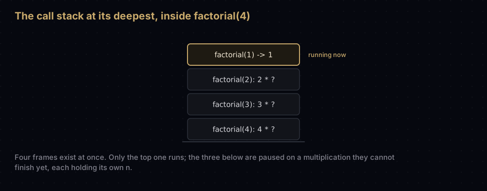
That picture is the entire mystery. factorial(4) cannot finish its multiplication until it knows factorial(3), so it sits there holding the number 4 while a new frame runs. Four frames exist at once, each with its own private n. Nothing is shared, nothing is overwritten.
Two rules follow, and every recursion bug is a violation of one of them:
- The base case must exist and must be reachable. Not just present in the source — actually reached by the arguments you pass.
- Every recursive call must move strictly closer to it.
factorial(n - 1)shrinks.factorial(n)does not. Neither doesfactorial(n - 1)whennis negative and the base test isn == 1.
Watching it work
Trace factorial(4) by hand. Going down, each call defers its multiplication:
factorial(4) = 4 * factorial(3)      frame 1 opens, holds 4
factorial(3) = 3 * factorial(2)      frame 2 opens, holds 3
factorial(2) = 2 * factorial(1)      frame 3 opens, holds 2
factorial(1) = 1                     frame 4 hits the base case
Nothing has been multiplied yet. Four frames are open and three of them are stuck on a half-written expression. Then the base case returns and the stack unwinds, in exactly the reverse order:
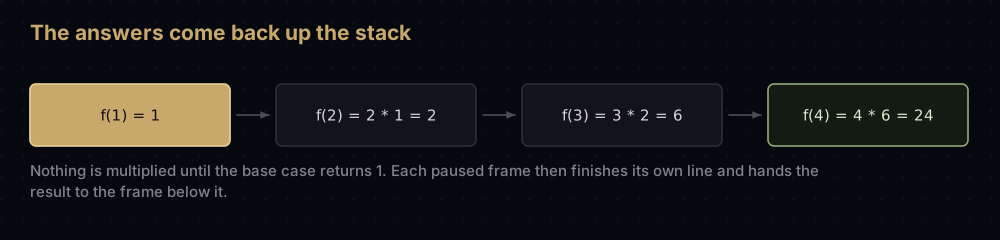
factorial(1) hands 1 back to factorial(2), which finally computes 2 × 1 = 2 and hands that to factorial(3), which computes 3 × 2 = 6, which lets factorial(4) compute 4 × 6 = 24. The work happens on the way up, not on the way down. That asymmetry is worth remembering. It is why a recursive function can build an answer in an order you never explicitly wrote.
Fibonacci changes the picture in one important way: the recursive case calls itself twice. fib(n) is fib(n - 1) + fib(n - 2), with fib(0) = 0 and fib(1) = 1. One call per level becomes a branching tree of calls.
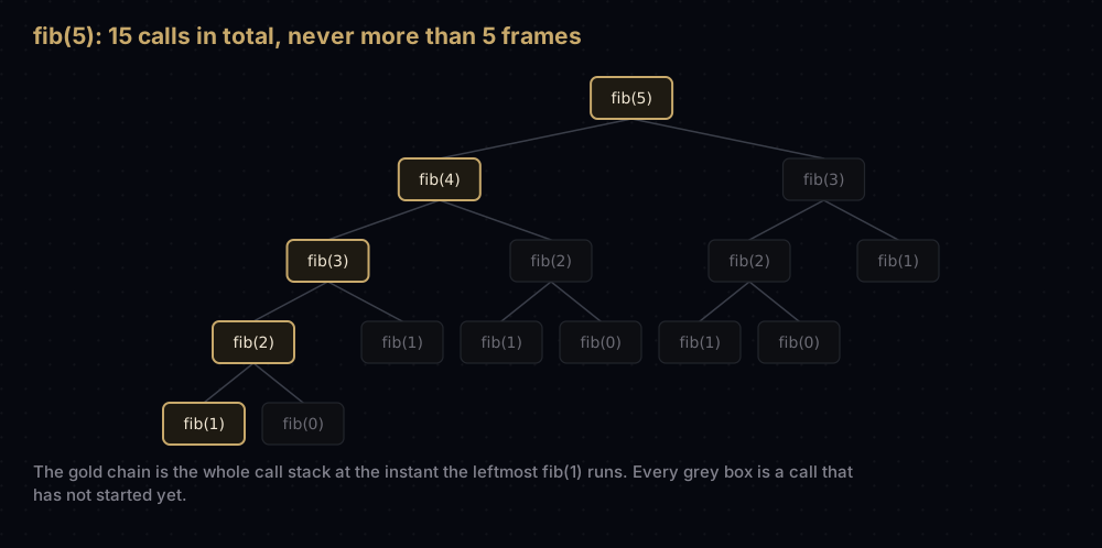
Fifteen calls in total to compute fib(5). But look at the highlighted chain: at the instant the leftmost fib(1) is running, only five frames exist. The other ten calls have not started yet. That distinction matters:
- Total calls determine the running time. For
fibthey explode. - Maximum depth determines the memory, because that is the tallest the stack ever gets. For
fibit is only n.
Count them separately, because they diverge. fib(30) makes 2,692,537 calls in a stack only 30 frames tall and runs fine; factorial(2000) makes 2,000 calls in a stack 2,000 frames tall and crashes.
The code
Factorial first, exactly as described:
def factorial(n: int) -> int:
    """n! computed from its own definition: n times the factorial below it."""
    if n <= 1:  # base case: 0! and 1! are both 1, and neither needs recursion
        return 1
    return n * factorial(n - 1)  # recursive case: the same job, one size smaller


print(factorial(4))
print([factorial(k) for k in range(7)])24
[1, 1, 2, 6, 24, 120, 720]If you do not yet believe the stack diagram, make the function narrate itself. Indentation here is literally the stack depth:
def factorial_traced(n: int, depth: int = 0) -> int:
    """factorial again, announcing each frame as it opens and as it returns."""
    pad = "  " * depth
    print(f"{pad}call factorial({n})")
    if n <= 1:
        print(f"{pad}base case, return 1")
        return 1
    result = n * factorial_traced(n - 1, depth + 1)
    print(f"{pad}return {n} * factorial({n - 1}) = {result}")
    return result


factorial_traced(4)call factorial(4)
call factorial(3)
call factorial(2)
call factorial(1)
base case, return 1
return 2 * factorial(1) = 2
return 3 * factorial(2) = 6
return 4 * factorial(3) = 24Four calls down, four returns up, and every return line is a frame finishing the multiplication it started. Printing a traced version of a recursion you do not understand is the fastest debugging technique in this entire series.
Now Fibonacci, with a second function that counts the calls instead of guessing at them:
def fib(n: int) -> int:
    """The nth Fibonacci number, written straight from the definition."""
    if n < 2:  # fib(0) = 0 and fib(1) = 1 are given, not computed
        return n
    return fib(n - 1) + fib(n - 2)


def fib_call_count(n: int) -> int:
    """Total calls the function above makes while computing fib(n)."""
    if n < 2:
        return 1
    return 1 + fib_call_count(n - 1) + fib_call_count(n - 2)


for k in (5, 10, 20, 30):
print(f"fib({k:>2}) = {fib(k):>6} calls: {fib_call_count(k):>9} deepest stack: {k}")fib( 5) = 5 calls: 15 deepest stack: 5
fib(10) = 55 calls: 177 deepest stack: 10
fib(20) = 6765 calls: 21891 deepest stack: 20
fib(30) = 832040 calls: 2692537 deepest stack: 30Adding ten to n multiplies the calls by about 123 while the stack grows by ten frames. Correct, and unusable past about n = 35. The fix is not to abandon recursion. It is to stop recomputing answers you already have, which is dynamic programming, and in Python it is one decorator: functools.lru_cache.
How the code maps to the idea
The base test comes first. Always. If the recursive call is written above the base test, the call happens before the test can stop it, and nothing stops it.
n - 1 is the contract. Each call receives an argument strictly closer to the base case, and the base case catches everything at or below the boundary. Writing if n == 1 instead of if n <= 1 looks equivalent and is not: factorial(0) then recurses to −1, −2, −3 and never matches.
The return value is the only channel. Each frame gets one value back from the frame above it and is responsible for turning that into its own answer. factorial multiplies. fib adds. Merge sort merges. That final combining step is where a divide-and-conquer algorithm actually does its work.
fib is exponential because the branches overlap, not because it recurses. fib(5) computes fib(3) twice, fib(2) three times, fib(1) five times. Recursion is not slow. Recomputation is slow.
Where recursion breaks
Delete the base case and something interesting happens: the program does not hang. It stops, quickly, with an exception.
import sys


def countdown(n: int) -> int:
    """No base case: every call makes another call, one frame deeper."""
    return countdown(n - 1)


try:
    countdown(5)
except RecursionError:
    print("countdown(5) stopped with RecursionError - it never hung")

print("frames allowed by default:", sys.getrecursionlimit())countdown(5) stopped with RecursionError - it never hung
frames allowed by default: 1000An infinite loop spins forever using no extra memory. An infinite recursion consumes a frame per call, so CPython counts frames and raises RecursionError at 1000 of them. That limit is a guard rail, not a law of nature — sys.setrecursionlimit(20000) raises it — but raise it only when the depth is genuinely bounded and merely larger than 1000. Frames are real memory, and on older CPython builds each Python call also consumed C stack, so a limit set high enough crashes the interpreter outright instead of raising a catchable exception.
The ceiling has one blunt consequence: a recursion whose depth grows with input size is a bug waiting for a big input. Walking a linked list of 5,000 nodes recursively passes your tests and dies in production.
Functional languages solve this with tail-call optimisation. A call is in tail position when it is the entire return expression — nothing is left to do after it comes back — so the compiler can reuse the current frame instead of stacking a new one. Scheme guarantees it. Python does not do it at all:
def sum_to(n: int, total: int = 0) -> int:
    """Tail recursive: the recursive call is the entire return expression."""
    if n == 0:
        return total
    return sum_to(n - 1, total + n)


print(sum_to(800))

try:
    print(sum_to(5000))
except RecursionError:
    print("sum_to(5000) overflows anyway - Python keeps every frame")


def sum_to_loop(n: int) -> int:
    """The same arithmetic as a loop: one frame, any n."""
    total = 0
    for value in range(1, n + 1):
        total += value
    return total


print(sum_to_loop(5000))
print(sum_to_loop(1_000_000))320400
sum_to(5000) overflows anyway - Python keeps every frame
12502500
500000500000sum_to is textbook tail recursion and it still blows the stack, while the loop handles a million in one frame. Guido van Rossum, Python's creator, wrote about this on his Neopythonic blog in 2009 and rejected the feature deliberately, not for lack of time. His main objection was debuggability: eliminating frames destroys the traceback, and a stack trace that has silently dropped its middle is a much worse tool than a slightly slower program. He also argued that Python is not a functional language, that iteration is the idiomatic way to loop, and that programmers should not have to reason about whether a call is in tail position to know whether their code will crash.
So in Python, the rule is blunt. Use recursion when the depth is naturally small: the height of a balanced tree, the number of digits in a number, log n levels of divide and conquer. Use a loop or an explicit stack when the depth scales with the data, which is exactly why the iterative version of depth-first search exists.
Backtracking: choose, explore, un-choose
Everything above computes a single value. Backtracking answers a different kind of question: enumerate every arrangement that satisfies some constraints, or find one that does.
The mechanism is three lines, repeated at every level:
- Choose. Commit to one option at the current position.
- Explore. Recurse to fill the next position, given that commitment.
- Un-choose. When the recursion returns, take the commitment back, so the next option starts from a clean state.
The un-choose step is the whole trick, and it is what makes this backtracking rather than plain recursion. The recursion explores one branch to its very end, then rewinds to the last decision point and takes the other road: depth-first search over a tree of decisions that you never build in memory. The tree exists only as the sequence of calls.
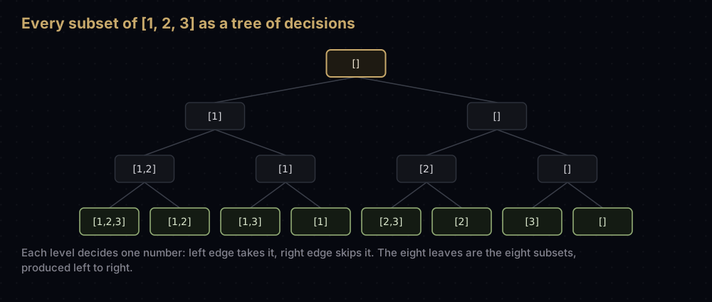
Start with subsets. To list every subset of [1, 2, 3] you decide, for each element in turn, take it or leave it. Three elements, two choices each, 2³ = 8 subsets.
def subsets(items: list[int]) -> list[list[int]]:
    """Every subset of items, by taking or leaving each element in turn."""
    result: list[list[int]] = []
    path: list[int] = []

    def explore(index: int) -> None:
        if index == len(items):
            result.append(list(path))  # copy, because path keeps changing
            return
        path.append(items[index])  # choose items[index]
        explore(index + 1)         # explore every ending that includes it
        path.pop()                 # un-choose, putting path back as it was
        explore(index + 1)         # explore every ending that leaves it out

    explore(0)
    return result


print(subsets([1, 2, 3]))
print(len(subsets([1, 2, 3, 4, 5])))[[1, 2, 3], [1, 2], [1, 3], [1], [2, 3], [2], [3], []]
32Read the output against the diagram: the leaves come out left to right, take-branch first. index == len(items) is the base case: every element has been decided, so the path is a finished subset. path.append is the choice, path.pop is the undo, and the two explore calls are the two branches out of every node.
Permutations, and one list rewound
Permutations are the same pattern with a different constraint. Instead of two choices per position, every unused element is a candidate, and each element must be used exactly once.
from itertools import permutations as stdlib_permutations


def permutations(items: list[int]) -> list[list[int]]:
    """Every ordering of items, choosing one unused element per position."""
    result: list[list[int]] = []
    path: list[int] = []
    used = [False] * len(items)

    def explore() -> None:
        if len(path) == len(items):
            result.append(list(path))
            return
        for index, value in enumerate(items):
            if used[index]:  # each element fills exactly one position
                continue
            used[index] = True   # choose
            path.append(value)
            explore()            # explore
            path.pop()           # un-choose, both halves of the state
            used[index] = False

    explore()
    return result


print(permutations([1, 2, 3]))
print(len(permutations([1, 2, 3, 4, 5, 6])))
print(permutations("abc") == [list(p) for p in stdlib_permutations("abc")])[[1, 2, 3], [1, 3, 2], [2, 1, 3], [2, 3, 1], [3, 1, 2], [3, 2, 1]]
720
TrueThat last True says the hand-written function produces the same orderings in the same order as itertools.permutations. In real code use the standard library version: it is written in C and yields results lazily instead of building a list of 720. Write your own when the constraints are custom, which is exactly when backtracking earns its place.
Notice that two things get undone in the loop: path.pop() and used[index] = False. Every piece of state you mutate on the way down has to be restored on the way up. Miss one and later branches inherit a corrupted world.
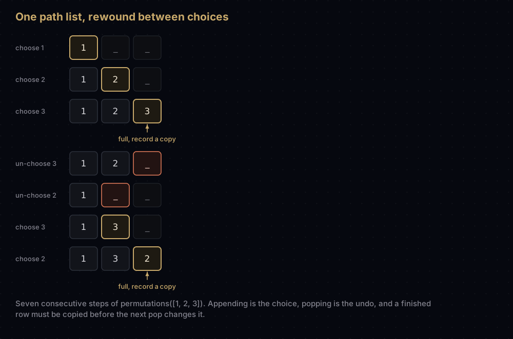
That diagram answers the question everyone asks eventually: when do you copy, and when do you mutate and undo?
- Mutate and undo the working state. There is one
pathlist for the entire search, and oneusedarray. Appending is amortised O(1), popping is O(1), and no new list is allocated per node. This is why backtracking is fast despite visiting a huge number of nodes. - Copy when you record an answer.
result.append(list(path))makes a snapshot. Writingresult.append(path)instead stores a reference to the one shared list, which keeps changing, so at the end every entry inresultis the same object, andsubsets([1, 2, 3])returns eight empty lists. This is the single most common backtracking bug. - Copy when you pass state down only if you cannot undo it cleanly. Passing
path + [value]into the recursive call is correct and much easier to reason about, but it allocates a new list at every node, which turns O(1) per node into O(n).
Pruning: not exploring what cannot work
So far the search visits everything. Backtracking becomes powerful when you check the constraints during the descent and abandon a branch the moment it cannot lead to a solution. Every node you skip takes its whole subtree with it.
Take a concrete problem: given twelve parcel weights, find every subset weighing exactly 60 kg. The plain version decides take-or-leave for each parcel and checks the total at the leaf. The pruned version stops at any node where the running total has already passed 60 (weights are positive, so it can only grow) or where everything still undecided adds up to less than what is still needed.
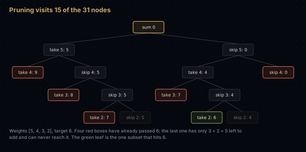
The diagram uses four weights so it fits on a page. [5, 4, 3, 2] with target 6 has a full tree of 31 nodes; the five abandoned branches shown remove 16 of them, leaving 15 visited, and the single solution [4, 2] is still found. Here are both versions on the twelve-parcel problem, counting nodes:
PARCELS = [31, 27, 15, 42, 8, 19, 23, 11, 37, 5, 14, 29]


def subsets_summing_to(weights: list[int], target: int) -> tuple[list[list[int]], int]:
    """Every subset that sums to target, exploring all 2**n leaves."""
    found: list[list[int]] = []
    nodes = 0

    def explore(index: int, path: list[int], total: int) -> None:
        nonlocal nodes
        nodes += 1
        if index == len(weights):
            if total == target:
                found.append(list(path))
            return
        path.append(weights[index])
        explore(index + 1, path, total + weights[index])
        path.pop()
        explore(index + 1, path, total)

    explore(0, [], 0)
    return found, nodes


def subsets_summing_to_pruned(weights: list[int], target: int) -> tuple[list[list[int]], int]:
    """The same answers, abandoning branches that provably cannot work."""
    # remaining[index] is the sum of everything from index onwards: the most
    # that can still be added once the first index parcels are decided.
    remaining = [0] * (len(weights) + 1)
    for index in range(len(weights) - 1, -1, -1):
        remaining[index] = remaining[index + 1] + weights[index]

    found: list[list[int]] = []
    nodes = 0

    def explore(index: int, path: list[int], total: int) -> None:
        nonlocal nodes
        nodes += 1
        if total > target:  # weights are positive, so the total only grows
            return
        if total + remaining[index] < target:  # not enough left to reach target
            return
        if index == len(weights):
            if total == target:
                found.append(list(path))
            return
        path.append(weights[index])
        explore(index + 1, path, total + weights[index])
        path.pop()
        explore(index + 1, path, total)

    explore(0, [], 0)
    return found, nodes


for target in (60, 25):
    plain, plain_nodes = subsets_summing_to(PARCELS, target)
    pruned, pruned_nodes = subsets_summing_to_pruned(PARCELS, target)
    print(f"target {target}: nodes {plain_nodes} -> {pruned_nodes} with pruning, "
          f"solutions {len(plain)}, identical answers: {plain == pruned}")

found, nodes = subsets_summing_to_pruned([5, 4, 3, 2], 6)
print(f"the diagram's tree: {found} found in {nodes} nodes instead of 31")target 60: nodes 8191 -> 929 with pruning, solutions 9, identical answers: True
target 25: nodes 8191 -> 141 with pruning, solutions 1, identical answers: True
the diagram's tree: [[4, 2]] found in 15 nodes instead of 31Same answers, 8,191 nodes down to 929. Target 25 does better still, at 141 nodes, because the first parcel weighs 31: taking it is already over target, so the take-it half of the tree collapses to the single node that gets rejected at depth 1 and its 4,094 descendants are never visited. Pruning pays most when it fires near the root, where the subtrees it discards are largest.
Be honest about what pruning buys, though. It does not change the growth rate. There are still 2ⁿ subsets, and an input where nothing can be ruled out early walks the whole tree. Pruning turns "impossible" into "fast enough for the inputs I actually have", which is usually what you need and never a guarantee.
Complexity
For any recursion, two independent quantities:
Time = number of calls × work per call. Count the calls with the recurrence the function itself describes.
factorial(n)makes exactly n calls, each doing one multiplication: O(n).fib(n)makes2 × fib(n + 1) − 1calls. Fibonacci numbers grow like φⁿ where φ ≈ 1.618, so this is O(1.618ⁿ), loosely quoted as O(2ⁿ). The measured numbers above confirm it: 21,891 calls at n = 20 and 2,692,537 at n = 30, a factor of 123 for ten extra terms, and 1.618¹⁰ ≈ 123.subsets(items)visits 2ⁿ⁺¹ − 1 nodes — a full binary tree of n + 1 levels, and copies an average of n/2 elements at each of its 2ⁿ leaves. The copying dominates: O(n · 2ⁿ). You cannot do better, because the output itself contains that many numbers.permutations(items)produces n! results and scans all n candidates at each of the n levels: O(n · n!).
Space = maximum stack depth × frame size, plus the shared state. This is where beginners overestimate the cost.
factorial(n)andsum_to(n)reach depth n: O(n) stack. That is the reason both hitRecursionError.fib(n)reaches depth n despite making exponentially many calls: O(n) stack.subsetsandpermutationsreach depth n and hold onepathof at most n elements: O(n) working space, plus whatever the collected results occupy.
For divide-and-conquer recursions that halve the input (binary search, merge sort) the depth is log₂ n, which is 20 for a million items and 30 for a billion. That is why those algorithms recurse safely in Python and a linked-list walk does not.
When to use it, and when not to
Use recursion when the problem is defined in terms of itself and the depth is bounded. Trees, nested structures like JSON, grammars, divide and conquer. A recursive tree traversal is six lines and obviously correct; the iterative one needs a stack, a visited marker and careful ordering.
Use backtracking when you must search combinations under constraints and there is no formula, no greedy rule and no polynomial algorithm. Sudoku, N-Queens, crossword filling, timetabling, exact set cover.
Do not use recursion when the depth scales with input size past a few hundred; convert it to a loop or keep an explicit list as your stack. Do not use plain recursion when subproblems repeat: add functools.lru_cache or rewrite it as dynamic programming, which is the difference between 2,692,537 calls and 31 distinct subproblems.
Do not use backtracking when a cheaper structure exists. Subset-sum over small integers is a dynamic programming table. Shortest paths are Dijkstra. Permutations are itertools. Backtracking should be a considered choice, not a reflex.
Where it shows up in the real world
Parsers. CPython's own parser is recursive descent: PEP 617 replaced the old LL(1) grammar with a PEG parser in Python 3.9, and PEG parsing backtracks by design, trying alternatives in order and rewinding the input position when one fails. The standard library's JSON decoder is recursive too, in both its C and its pure-Python scanner, which is why json.loads on a deeply nested document raises RecursionError.
Regular expressions. Python's re module is a backtracking engine. a* first grabs as much as it can, and if the rest of the pattern then fails, it gives a character back and retries: choose, explore, un-choose, over the characters of a string. The same idea in twelve lines, matching glob patterns:
def matches(pattern: str, text: str) -> bool:
    """Glob-style matching where '?' is any one character and '*' is any run."""
    if not pattern:
        return not text
    if pattern[0] == "*":
        # Let the star match nothing; if the rest of the pattern then fails,
        # backtrack and hand the star one more character.
        return matches(pattern[1:], text) or (bool(text) and matches(pattern, text[1:]))
    if not text:
        return False
    if pattern[0] in ("?", text[0]):
        return matches(pattern[1:], text[1:])
    return False


for pattern, text in [("*.py", "main.py"), ("*.py", "main.txt"),
                      ("a*c", "abbbc"), ("a?c", "ac"), ("*x*y*", "axolotly")]:
print(f"{pattern:6} vs {text:9} -> {matches(pattern, text)}")*.py vs main.py -> True
*.py vs main.txt -> False
a*c vs abbbc -> True
a?c vs ac -> False
*x*y* vs axolotly -> TrueThe or is the backtrack: try the shorter match, and only if the whole rest of the pattern fails does the star swallow another character. The standard library equivalent is fnmatch.fnmatch, which works by translating the glob into a regex. The cost of that same mechanism is real: in 2016 Stack Overflow was taken offline for 34 minutes by catastrophic backtracking in a single regular expression scanning a post with a very long run of whitespace. Backtracking engines can go exponential on innocent-looking patterns.
Constraint satisfaction and SAT solvers. The DPLL algorithm from 1962, still the skeleton inside modern SAT solvers, is backtracking search over variable assignments with propagation as its pruning rule. Prolog's entire execution model is backtracking. Sudoku solvers, exam timetablers and puzzle generators are all the same shape: choose a value for the next empty slot, check the constraints, explore, undo.
Nested data. A directory tree, an HTML document and a JSON object are recursive structures, so the code that walks them is recursive too: shutil.rmtree descends into each subdirectory by calling itself, and every tree algorithm in this series does the same.
Common mistakes
No base case, or an unreachable one. if n == 1 misses n = 0 and every negative number. Test the boundary: factorial(0), subsets([]), an empty tree.
Recursing on the same size. factorial(n) inside factorial compiles fine and dies with RecursionError. Every call must strictly shrink the problem.
Storing the shared path instead of a copy. result.append(path) gives you a list of identical, mutated lists. result.append(list(path)) is the fix.
Forgetting to undo part of the state. Popping path but leaving used[index] = True marks every element consumed forever, so the search never backs up past its first descent: permutations([1, 2, 3]) returns [[1, 2, 3]] and nothing else, one ordering instead of six. Undo everything you did, in the reverse order you did it.
Assuming recursion is why your code is slow. Usually it is recomputation. Add functools.lru_cache before rewriting anything as a loop, and measure.
Returning nothing from the recursive branch. Writing factorial(n - 1) instead of return n * factorial(n - 1) makes the function return None: a bug that Python reports far away from where it happened.
Practice
- Write a recursive function that reverses a string, with the empty string as the base case.
- Write a recursive
count_leavesfor a nested list such as[1, [2, [3, 4]], 5], then state its maximum stack depth. - Convert
factorialinto a loop, and confirm both agree for every n from 0 to 20. - Generate all subsets of size exactly k by pruning any branch whose path is already longer than k.
- Write a Sudoku solver: find the first empty cell, try digits 1 to 9, keep any digit that breaks no row, column or box constraint, recurse, and undo it if the recursion fails.
Summary
Recursion is two parts and one data structure: a base case, a strictly smaller recursive case, and the call stack that remembers everything half-finished. Backtracking adds one line — undo the last choice — and turns that stack into a systematic search over every arrangement, with pruning as the lever that makes it practical. Count calls for time, count depth for space, and remember that Python gives you 1000 frames and no tail-call optimisation, so depth is a design constraint rather than a detail.
| Difficulty | Medium |
| Time, linear recursion | O(n) — one call per level, as in factorial |
| Time, branching recursion | O(bᵈ) — b calls per level, d levels deep, so fib is O(1.618ⁿ) |
| Time, full enumeration | O(n · 2ⁿ) for all subsets, O(n · n!) for all permutations |
| Space | O(depth) — one frame per open call, plus one shared path |
| Python depth limit | 1000 frames by default, from sys.getrecursionlimit() |
| Tail-call optimisation | None, and deliberately so — it would destroy tracebacks |
| Data structure | The call stack, plus one mutable path list you undo |
| Use it when | The problem is self-similar, or you must enumerate under constraints |
| Avoid it when | Depth grows with input size, or subproblems repeat — loop or memoize |
| Real-world use | Recursive descent and PEG parsers, regex engines, SAT and CSP solvers |
| Python equivalents | itertools.permutations, functools.lru_cache, re, fnmatch |
Keep reading
- Dynamic Programming — the fix for the exponential
fibabove, in one decorator or one table. - The N-Queens Problem — backtracking with real constraints, and the clearest pruning you will see.
- Depth-First Search — the same descent applied to a graph, both recursively and with an explicit stack.
- Stacks — what the call stack actually is, and how to build your own when recursion runs out of frames.
- Merge Sort — divide and conquer, where recursion depth is log n and the combining step is the algorithm.


