Dynamic programming has a reputation for being the hardest topic in algorithms. It is actually one of the smallest. It is a single observation applied relentlessly: if your program works out the same answer twice, work it out once and write it down.
The gap that one observation closes is enormous. The textbook recursive Fibonacci function makes 40,730,022,147 calls to compute fib(50), which is roughly an hour of CPython on a modern laptop. The same recursion with a dictionary bolted onto it makes 99 calls and returns instantly. Nothing about the recursion changed: only the bookkeeping around it.
The name is unhelpful, so ignore it. Richard Bellman coined "dynamic programming" at RAND in the 1950s and, by his own account, picked a name that would not read as mathematical research to a defense secretary who was hostile to the word. "Programming" there means planning and scheduling, not writing code.
The idea
Fibonacci is defined by three lines. fib(0) is 0, fib(1) is 1, and every later term is the sum of the two before it: fib(n) = fib(n - 1) + fib(n - 2). Translating that into Python takes about as long as reading it.
def fib_naive(n: int) -> int:
    """Fibonacci written exactly as its mathematical definition reads."""
    if n < 2:  # fib(0) = 0 and fib(1) = 1 are given, not derived
        return n
    return fib_naive(n - 1) + fib_naive(n - 2)


print([fib_naive(i) for i in range(10)])
print(fib_naive(25))[0, 1, 1, 2, 3, 5, 8, 13, 21, 34]
75025That function is correct and, past about n = 35, unusable. To see why, draw the calls it makes: fib(5) triggers fib(4) and fib(3), fib(4) triggers fib(3) and fib(2), and so on until everything bottoms out at fib(1) or fib(0).
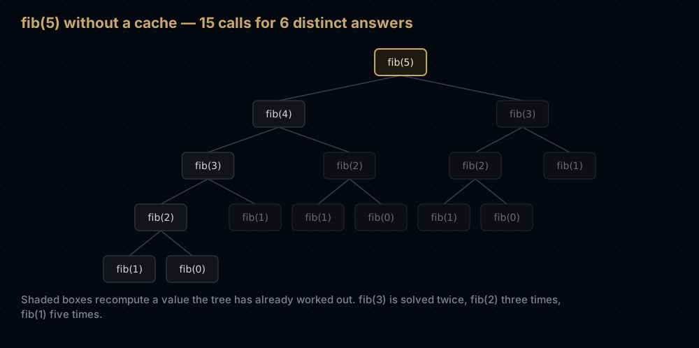
Fifteen boxes, and only six of them ask a question that has not already been answered: fib(5), fib(4), fib(3), fib(2), fib(1) and fib(0). The other nine are pure waste. fib(3) is computed twice from scratch, fib(2) three times, fib(1) five times, and the ratio gets worse fast.
That picture is the whole motivation. Two facts follow from it, and they are the two halves of dynamic programming:
- The subproblems overlap. The same question is asked over and over, in different branches of the tree.
- A big answer is built from smaller ones. Once you know
fib(4)andfib(3)you knowfib(5), and nothing about how you got those two numbers matters.
When both hold, you can solve each distinct subproblem once, store the answer, and hand it out on every later request.
Watching it work
Count the waste rather than eyeballing it. The number of calls follows its own recurrence: computing fib(n) is one call plus everything fib(n - 1) costs plus everything fib(n - 2) costs, so C(n) = 1 + C(n - 1) + C(n - 2), with C(0) = C(1) = 1.
def measured_calls(n: int) -> int:
    """Run the naive recursion with a counter attached and report the total."""
    calls = 0

    def walk(k: int) -> int:
        nonlocal calls
        calls += 1
        if k < 2:
            return k
        return walk(k - 1) + walk(k - 2)

    walk(n)
    return calls


def predicted_calls(n: int) -> int:
    """The same total from the recurrence C(n) = 1 + C(n - 1) + C(n - 2)."""
    if n < 2:
        return 1
    older, newer = 1, 1  # C(0) and C(1)
    for _ in range(n - 1):
        older, newer = newer, 1 + newer + older
    return newer


print(f"{'n':>2} {'measured':>10} {'predicted':>11}")
for n in range(7):
    print(f"{n:>2} {measured_calls(n):>10} {predicted_calls(n):>11}")

for n in (20, 30, 40, 50):
print(f"fib({n}) would make {predicted_calls(n):,} calls") n measured predicted
0 1 1
1 1 1
2 3 3
3 5 5
4 9 9
5 15 15
6 25 25
fib(20) would make 21,891 calls
fib(30) would make 2,692,537 calls
fib(40) would make 331,160,281 calls
fib(50) would make 40,730,022,147 callsThe counter agrees with the recurrence, and fib(5) really does cost 15 calls: the fifteen boxes in the diagram. Now look at the ratios: 2,692,537 divided by 21,891 is 123, and 331,160,281 divided by 2,692,537 is also 123. Ten extra steps of n multiply the work by 123, so one extra step multiplies it by about 1.618. That is the golden ratio, and it is no coincidence: C(n) equals 2 · fib(n + 1) - 1, and Fibonacci numbers grow by a factor of the golden ratio per step. The naive recursion is exponential.
Now add the cache. Same recursion, same order of calls, but a call whose answer is already stored returns immediately instead of expanding into a subtree.
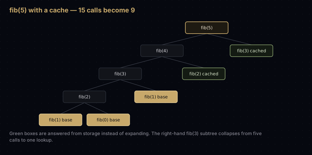
The right-hand fib(3) was a five-node subtree; it is now a single box that reads a stored value, and the tree collapses from fifteen boxes to nine. Count that for larger n:
def measured_memo_calls(n: int) -> int:
    """How many times the recursion is entered once answers are remembered."""
    calls = 0
    cache: dict[int, int] = {}

    def walk(k: int) -> int:
        nonlocal calls
        calls += 1
        if k < 2:
            return k
        if k not in cache:
            cache[k] = walk(k - 1) + walk(k - 2)
        return cache[k]

    walk(n)
    return calls


print(f"{'n':>3} {'naive calls':>14} {'with a cache':>14}")
for n in (5, 10, 20, 30, 50):
print(f"{n:>3} {predicted_calls(n):>14,} {measured_memo_calls(n):>14}") n naive calls with a cache
5 15 9
10 177 19
20 21,891 39
30 2,692,537 59
50 40,730,022,147 99The cached column is exactly 2n - 1. The reason is easy to see: each of the n − 1 non-base subproblems is expanded exactly once and makes exactly two calls, giving 2(n − 1) calls, plus the one call at the top. Exponential became linear, and the code barely changed.
The two conditions
Dynamic programming applies when a problem has both of these. Neither alone is enough.
Overlapping subproblems. Solving the problem naively asks the same smaller question more than once. Fibonacci asks for fib(3) twice at n = 5 and 4,807,526,976 times at n = 50. Without overlap there is nothing to cache and the cache is pure overhead.
Optimal substructure. An optimal answer to the whole problem contains optimal answers to its subproblems. Shortest paths have it: if the shortest route from Pokhara to Kathmandu goes through Mugling, the piece from Pokhara to Mugling must itself be the shortest route between those two towns — otherwise you could swap in a shorter piece and beat the supposedly shortest whole. That is what lets you combine sub-answers without re-examining how they were built.
Each condition can fail on its own, and seeing that is what tells you when to stop reaching for DP.
Optimal substructure without overlap: merge sort. Splitting a list in half, sorting each half and merging has perfect optimal substructure. But the two halves are disjoint, so no subproblem is ever asked for twice, and caching sorted sublists would burn memory to save nothing. That is divide and conquer — the same recursive shape without the repetition.
Overlap without optimal substructure: the longest simple path. A simple path never revisits a vertex. Ask for the longest simple path between two vertices of this graph:
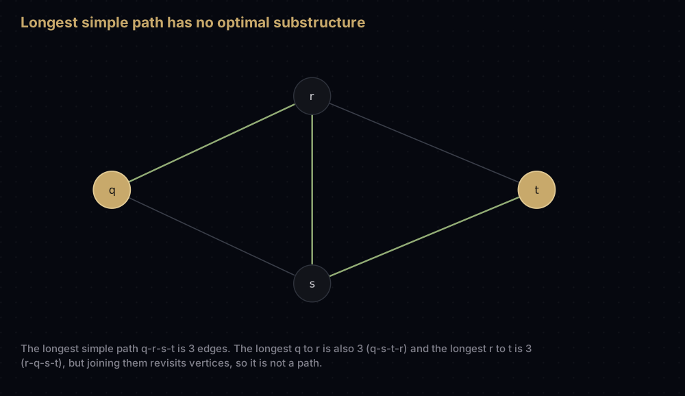
The longest simple path from q to t is three edges: q, r, s, t. Now try to build it the way DP would, by splitting at r. The longest simple path from q to r is also three edges (q, s, t, r), and the longest from r to t is three as well: r, q, s, t. Gluing those gives six edges, but the result revisits q, s and t, so it is not a path at all. The optimal whole is not made of optimal parts. Subproblems overlap heavily here and it does not help: finding the longest simple path in a general graph is NP-hard, and caching does not change that. Restrict the graph to a directed acyclic one and optimal substructure comes back, which is exactly why longest-path DP works on DAGs and not on general graphs.
The code
There are two ways to write down the same recurrence. Both compute the same answer from the same base cases, and differ in who drives the loop.
Top-down: memoization
Keep the recursion exactly as written and put a dictionary in front of it. This is memoization: recursion plus a lookup table.
def fib_memo(n: int) -> int:
    """Top-down Fibonacci: the same recursion, with every answer remembered.

    The cache lives in the enclosing call rather than in a default argument.
    A mutable default is built once when the function is defined and then
    shared by every caller for the lifetime of the program.
    """
    cache: dict[int, int] = {}

    def solve(k: int) -> int:
        if k < 2:
            return k
        if k not in cache:
            cache[k] = solve(k - 1) + solve(k - 2)
        return cache[k]

    return solve(n)


print(fib_memo(25))
print(fib_memo(90))75025
2880067194370816120Three lines carry the idea. if k not in cache stops the subtree expanding a second time. cache[k] = ... records the answer on the way back up. return cache[k] serves the freshly computed case and the cache hit alike. Base cases return before touching the cache, because they are cheaper to recompute than to look up.
Let the standard library do it
Python ships memoization as a decorator. functools.cache (Python 3.9 and later) is an unbounded dictionary keyed on the arguments; functools.lru_cache(maxsize=...) is the same thing with a size cap that evicts the least recently used entry. Both require the arguments to be hashable.
from functools import cache


@cache
def fib_cached(n: int) -> int:
    """Identical recursion; functools.cache supplies and manages the dictionary."""
    if n < 2:
        return n
    return fib_cached(n - 1) + fib_cached(n - 2)


print(fib_cached(100))
print(fib_cached.cache_info())

try:
    fib_cached(3000)
    print("fib_cached(3000) returned a number")
except RecursionError:
print("fib_cached(3000) hit Python's recursion limit")354224848179261915075
CacheInfo(hits=98, misses=101, maxsize=None, currsize=101)
fib_cached(3000) hit Python's recursion limitcache_info() is the honest report on your DP. 101 misses means 101 distinct subproblems were solved, one for each of fib(0) through fib(100); 98 hits means 98 calls were answered from storage. Misses count states, hits count avoided work.
The last three lines show the catch. Top-down DP recurses as deep as the longest chain of subproblems, and CPython's default recursion limit is 1,000 frames, so fib_cached(3000) dies before the cache can help. Raising sys.setrecursionlimit moves the wall without removing it, because the real limit is the C stack.
Bottom-up: tabulation
Turn the recursion inside out. Instead of asking for fib(n) and letting it request smaller values, start at the base cases and fill an array upward. This is tabulation.
def fib_table(n: int) -> list[int]:
    """Bottom-up Fibonacci: fill a table upward, starting from the base cases.

    Returns the whole table so the filling order stays visible; ``table[n]``
    is the answer.
    """
    table = [0] * (n + 1)
    if n >= 1:
        table[1] = 1
    for i in range(2, n + 1):
        # Both operands were written on earlier iterations, so they are ready.
        table[i] = table[i - 1] + table[i - 2]
    return table


print(fib_table(7))
print(fib_table(0))[0, 1, 1, 2, 3, 5, 8, 13]
[0]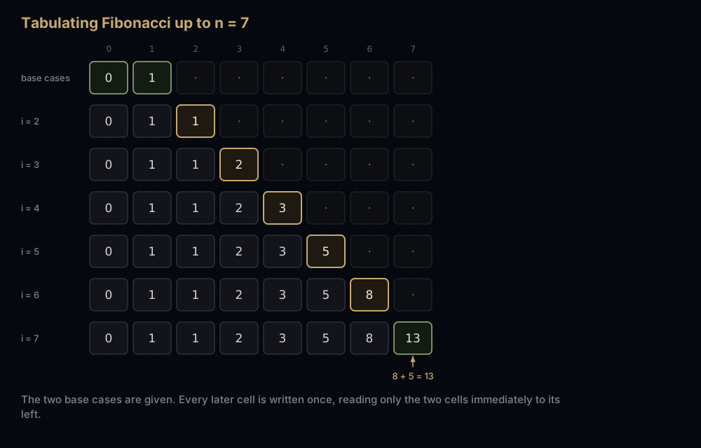
No recursion, no stack, no dictionary: a list and a single loop. The if n >= 1 guard exists because fib_table(0) must not write to table[1], which does not exist, and the loop starting at 2 is the base-case boundary made explicit.
The decision that matters here is the iteration order. table[i] reads table[i - 1] and table[i - 2], so i must increase. Reverse it and you read zeros that have not been written yet: a wrong answer rather than an error. In tabulation the loop order is part of the algorithm, not a stylistic choice.
Top-down or bottom-up
Both are correct. The choice between them is a real trade-off.
Top-down wins when the state space is sparse. Recursion only visits states reachable from the question you asked; tabulation fills the whole table whether or not each cell matters. Count the ways to reach 10,000 using coins worth 250, 500 and 1,000:
def reachable_states(amount: int, coins: tuple[int, ...]) -> int:
    """Distinct remaining-amount states a top-down solver ever asks about."""
    seen: set[int] = set()

    def walk(left: int) -> None:
        if left < 0 or left in seen:
            return
        seen.add(left)
        for coin in coins:
            walk(left - coin)

    walk(amount)
    return len(seen)


print(f"bottom-up table entries: {10_000 + 1:>6}")
print(f"states top-down visits: {reachable_states(10_000, (250, 500, 1000)):>6}")bottom-up table entries: 10001
states top-down visits: 41Every reachable remaining amount is a multiple of 250, so there are 41 of them. A bottom-up table over every amount from 0 to 10,000 does about 244 times more work than necessary. Top-down also lets you transcribe the recurrence directly, which is far less error-prone on an unfamiliar problem.
Bottom-up wins on everything else. No recursion limit, so n can be a million. No per-call overhead — a Python function call costs far more than an array write, and top-down makes at least one call per state. And once the values sit in an array in a known fill order, you can see which parts are still needed, which is what makes space optimization possible.
The practical workflow: solve it top-down because that is easier to get right, then convert to bottom-up if the depth or the constant factor bites.
Shrinking the space
Look again at the Fibonacci loop. table[i] reads only table[i - 1] and table[i - 2], so everything older is dead weight. Keep two variables instead of an array of n + 1 numbers.
def fib_rolling(n: int) -> int:
    """Bottom-up Fibonacci keeping only the two table entries still in use."""
    previous, current = 0, 1  # fib(0) and fib(1)
    for _ in range(n):
        previous, current = current, previous + current
    return previous


print([fib_rolling(i) for i in range(10)])
print(fib_rolling(500) == fib_table(500)[500])[0, 1, 1, 2, 3, 5, 8, 13, 21, 34]
TrueO(n) space became O(1), and the answers still match the full table exactly. The rule generalizes: keep only the slice of the table your recurrence still reads. There is a cost: the intermediate values are gone, so if the problem asks which choices produced the answer, you need the full table or a separate parent-pointer array.
A two-dimensional table
The same trick applies one dimension up. Count the routes across a grid where you may only step right or down. A cell is entered from its left neighbor or from the cell above, so the routes into it are the sum of those two, and the top row and left column each have exactly one route.
def grid_paths(rows: int, cols: int) -> list[list[int]]:
    """Count the paths from the top-left cell of a grid to every other cell.

    Moves are one step right or one step down, so the only ways into a cell
    are from its left neighbor and from the cell directly above it.
    """
    table = [[1] * cols for _ in range(rows)]
    for row in range(1, rows):
        for col in range(1, cols):
            table[row][col] = table[row - 1][col] + table[row][col - 1]
    return table


for row in grid_paths(3, 4):
print(row)[1, 1, 1, 1]
[1, 2, 3, 4]
[1, 3, 6, 10]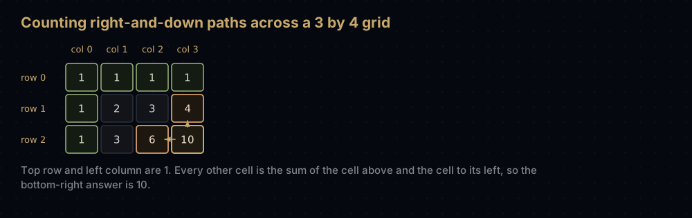
Ten routes across a 3 by 4 grid, and 6 = 3 + 3, 10 = 6 + 4, and so on. You can verify the whole table by eye in ten seconds, which is exactly the check worth doing before you trust a DP.
Now notice that row 2 reads only row 1, and row 0 is never touched again. One row of storage is enough, provided you overwrite it left to right: when you reach row[col] the entry still holds the value from the row above, and row[col - 1] already holds this row's value.
def grid_paths_rolling(rows: int, cols: int) -> int:
    """The same recurrence, keeping only the row currently being written."""
    row = [1] * cols
    for _ in range(rows - 1):
        for col in range(1, cols):
            # row[col] still holds the value from the row above, and
            # row[col - 1] already holds this row's value, which is exactly
            # the pair the recurrence adds together.
            row[col] += row[col - 1]
    return row[-1]


print(grid_paths_rolling(3, 4))
print(grid_paths_rolling(18, 18) == grid_paths(18, 18)[-1][-1])10
True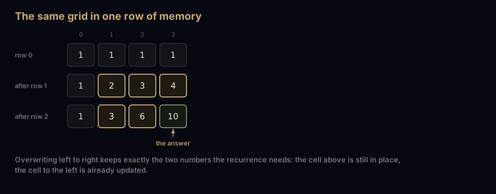
O(rows × cols) space became O(cols). The direction of that inner loop is load-bearing: it works because the recurrence reads the cell above and the cell to the left. When a recurrence reads the cell above and the cell up-left, as 0/1 knapsack does, the same in-place trick requires iterating the row backwards instead. Getting that direction wrong is the single most common bug in space-optimized DP.
Complexity
Every dynamic program has the same cost formula, and it turns complexity analysis into counting:
Time = (number of distinct states) × (work done per state). Space = the number of states you must keep alive at once, plus the recursion depth if you solved it top-down.
For Fibonacci the states are the values 0 through n, so there are n + 1 of them, and each does one addition and two dictionary or array reads. That is O(1) work per state, so O(n) time. Storage is one entry per state, so O(n) space, and the top-down version holds up to n stack frames on top of the cache, which is the same O(n). The rolling pair takes it to O(1). Compare that with the naive version's O(1.618ⁿ) and the improvement is not a constant factor, it is a change of growth class.
For grid paths there are rows × cols states and each is one addition, so O(rows × cols) time, and O(cols) space after the rolling-row rewrite.
Two honest caveats:
The "O(1) work per state" claim assumes arithmetic is free. For Fibonacci it is not: fib(n) has roughly 0.694n bits, so adding two of them costs O(n) bit operations. The linear bound counts additions; the true bit cost of the loop is quadratic. That never matters when values fit in a machine word, which is nearly always, but the distinction is what separates an analysis from a slogan.
Polynomial in the state count is not polynomial in the input. The 0/1 knapsack DP runs in O(n × W) for n items and capacity W. W is a value, though, and writing 1,000,000,000 takes ten digits, so the runtime is exponential in the length of the input. That is what pseudo-polynomial means. For the full treatment of these bounds, read Big O notation.
A recipe for any DP problem
Run these five steps in order. Doing them out of order is why DP feels hard.
- Identify the state. What is the smallest set of facts that fully determines the answer to a subproblem? For Fibonacci it is one number, n. For grid paths it is a pair, the row and the column. If two different situations share a state but have different answers, your state is incomplete: add the missing fact.
- Write the recurrence. Express the answer for a state in terms of strictly smaller states, in English first: "the routes into this cell are the routes into the cell above plus the routes into the cell to the left." The code follows from the sentence.
- Find the base cases. The states whose answers are given rather than derived. This is where off-by-one bugs live: check that the recurrence never runs below them.
- Decide the iteration order. Top-down, recursion picks the order for you. Bottom-up, you must fill each state only after everything it reads. For a 2D table that usually means both indices increasing, but check it against the recurrence from step 2 rather than assuming.
- Optimize the space, last. Once the full table is correct and tested, keep only the slices the recurrence still reads. Never do this before step 4 works, or you will not be able to tell a space bug from a logic bug.
On the grid: the state is (row, col); the recurrence is paths[row][col] = paths[row - 1][col] + paths[row][col - 1]; the base cases are the top row and left column, all 1; the order is rows then columns, both increasing; the space collapses to one row. Five answers, and the code writes itself.
When DP is the wrong tool
When a greedy rule provably works. If the locally best option always leads to the globally best answer, take it: greedy is faster and simpler. Change-making with coins worth 1, 5, 10 and 25 is greedy-solvable; with coins worth 1, 3 and 4 it is not, because greedy pays for 6 with 4 + 1 + 1 while the best answer is 3 + 3. Greedy algorithms covers how to tell the two apart.
When subproblems never repeat. Use divide and conquer and skip the cache.
When the state space is too large to enumerate. The traveling salesman DP over subsets of cities runs in O(2ⁿ · n²). That crushes the O(n!) brute force and is still hopeless at 60 cities. A state space you cannot afford to store is one DP cannot help with.
When the problem lacks optimal substructure, as with longest simple paths above. Caching a wrong recurrence just gives you wrong answers faster.
Where it shows up in the real world
- Diffing files.
git diffand GNUdiffuse Myers' algorithm, a shortest-path search over an edit graph: dynamic programming with a clever pruning rule. Every code review you have ever read was produced by a DP. - Spelling correction and fuzzy matching. Levenshtein edit distance is the Wagner-Fischer DP table. PostgreSQL exposes it directly as
levenshtein()in thefuzzystrmatchextension. - Sequence alignment in biology. Needleman-Wunsch (1970) for global alignment and Smith-Waterman (1981) for local alignment are DP tables over two sequences, still the exact-alignment reference that faster heuristics are measured against.
- Error-correcting codes and speech. The Viterbi algorithm finds the most likely sequence of hidden states by DP, and it decodes convolutional codes in GSM, 802.11 wireless and NASA's deep-space links.
- Typesetting. TeX breaks paragraphs into lines with the Knuth-Plass algorithm, a DP that minimizes total badness over every possible set of break points. It is why TeX paragraphs look better than the greedy line-breaking a web browser does.
- Database query planning. Choosing a join order is a DP over subsets of tables, an approach from IBM's System R in 1979. PostgreSQL still uses it, switching to a genetic search once a query reaches
geqo_thresholdrelations (12 by default). - Python itself.
functools.lru_cacheexists because memoization is useful often enough to belong in the standard library. Building an LRU cache shows what is inside it.
Common mistakes
A mutable default argument as the cache. def solve(n, cache={}) builds the dictionary once, when the function is defined, and shares it across every later call. If the answers depend on anything besides n (a different input list, a different target) you serve stale results. Build the cache inside a wrapper, or use functools.cache.
Caching on an incomplete state. If the answer depends on an index and a remaining capacity but you key on the index alone, later lookups return answers computed under different conditions. That is wrong output, not slow output, and it is the hardest DP bug to spot. Test the memoized version against the naive one on small inputs.
Passing unhashable arguments to lru_cache. A list argument raises TypeError: unhashable type: 'list'; convert it to a tuple. Decorating a method caches on self too, keeping every instance alive as long as the cache.
Filling the table in an order that reads unwritten cells. The default value masquerades as a real answer. Before writing the loops, list the cells the recurrence reads and confirm they are all behind the write.
Off-by-one in the table size. States 0 through n need n + 1 slots. [0] * n is the classic error, and it fails only at the very last cell.
Optimizing space too early, or in the wrong direction. Get the full table correct first. When you collapse it, check whether the recurrence reads the cell to the left (iterate forwards) or up-left (iterate backwards). Reverse that in 0/1 knapsack and a single item gets used twice.
Practice
- Count the ways to climb n stairs taking 1 or 2 steps at a time. Write it memoized and tabulated, then explain why the answers are Fibonacci numbers shifted by one.
- Given a list of house values, find the largest sum you can take without ever picking two adjacent houses. The state is one index; the recurrence has two branches.
- Redo the grid-path count with some cells blocked. Decide what a blocked cell's value should be, and check your rule against a grid whose first column is blocked halfway down.
- Given coin values and a target, find the fewest coins that make it, then separately count the distinct combinations that make it. The two differ only in loop order: work out which order does which, and why.
- Find the length of the longest increasing subsequence of a list in O(n²) using one state per index. Then read up on how
bisectreduces it to O(n log n) with a different formulation entirely.
Summary
Dynamic programming is not a category of problem, it is a response to a shape: a recursion whose tree repeats itself. Spot the repeat, name the state, write the recurrence, and the rest is bookkeeping. Memoization gets you there fastest; tabulation gets you further; the rolling window gets you cheaper. Every classic DP problem in this series (knapsack, longest common subsequence, edit distance, coin change) is that same recipe with a different state.
| Difficulty | Medium |
| Applies when | Subproblems overlap and optimal answers are built from optimal sub-answers |
| Time | O(states × work per state) — for Fibonacci, O(n) |
| Space | O(states kept alive) — often one row, sometimes two variables |
| Naive Fibonacci | O(1.618ⁿ) time — 2 · fib(n + 1) − 1 calls, 40.7 billion at n = 50 |
| Memoized Fibonacci | O(n) time, O(n) space — exactly 2n − 1 calls |
| Top-down | Recursion plus a cache; visits only reachable states; limited by stack depth |
| Bottom-up | Loops over a table; no depth limit, faster constants, easy to shrink |
| Data structure | Dict keyed on the state, or a list / list of lists |
| Use it when | The same subproblem is asked for more than once |
| Avoid it when | A greedy rule provably works, subproblems never repeat, or the states will not fit |
| Real-world use | git diff, Levenshtein spell-check, Viterbi decoding, TeX line breaking, SQL join ordering |
| Python equivalent | functools.cache / functools.lru_cache for instant memoization |
Write the naive recursion first, always. It is the specification, it is usually four lines, and it is what you test the fast version against. Everything after that is mechanical.
Keep reading
- Recursion and Backtracking — the call-stack model that top-down DP is built on, and how to read a recursion tree.
- The Coin Change Problem — the cleanest demonstration of greedy failing and DP winning, plus the two loop orders.
- The 0/1 Knapsack Problem — the two-dimensional table, and the backwards in-place trick this post warned about.
- Longest Common Subsequence — DP over two strings, and the algorithm behind diff tools.
- Edit Distance (Levenshtein) — three choices per cell instead of two, and how spell-checkers rank suggestions.


