
Merge sort makes a promise that no simple sorting algorithm can make: O(n log n) time on every input. Not on average, not when the data happens to be friendly. Every list, every time — random, reversed, already sorted, or deliberately constructed to be the worst possible case. That single guarantee is why merge sort is still in production code eighty years after John von Neumann wrote it down in 1945.
The guarantee costs something, and the honest version of this post says so early: merge sort needs O(n) extra memory. Quick sort is usually faster on data that fits in RAM and sorts in place; heap sort matches the O(n log n) bound with no extra memory at all. Merge sort's answers are that it is stable — items that compare equal come out in the order they went in — and that it is the only one of the three that still works when the data is far too big to fit in memory.
It is also the algorithm you are already running. Python's sorted() and list.sort() use Timsort, which is merge sort taught to recognise the sorted stretches that real data already contains. Understand merge sort and you are most of the way to understanding your standard library.
The idea
Merge sort is the cleanest example of divide and conquer, a strategy with three steps:
- Divide — cut the list into two halves. No comparing, no rearranging. Just split it down the middle.
- Conquer — sort each half. Do this by calling merge sort on it, which splits it again, and again, until you reach lists of one item. A one-item list is already sorted, so there is nothing left to do.
- Combine — take the two sorted halves and merge them into one sorted list.
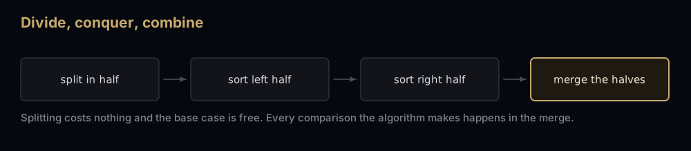
Steps 1 and 2 are almost free. Splitting a list in half requires no thought, and the recursion bottoms out immediately at lists of one element. All the real work is in step 3. The merge is the algorithm; everything else is scaffolding that arranges for the merge to be handed two sorted lists. So here it is on its own.
You have two sorted lists. Put a finger at the front of each. The smallest value in the combined result must be under one of your two fingers: nothing behind a finger can be smaller, because each list is sorted. So compare the two values under your fingers, take the smaller, write it to the output, and move that finger forward one place. Repeat.
Eventually one finger runs off the end of its list. Everything left under the other finger is already sorted, and is already larger than everything you have written out, so you copy the whole remainder across without comparing anything.
That procedure looks at each of the m combined items exactly once and writes it exactly once. Merging two sorted lists holding m items between them costs O(m) time and at most m − 1 comparisons. Hold on to that number; the whole complexity argument is built from it.
Watching it work
Sort [38, 27, 43, 3, 9, 82, 10].
Splitting
With seven items the middle is index 3, so the first split gives [38, 27, 43] and [3, 9, 82, 10]. Each half splits again, and again, until every piece holds a single value:
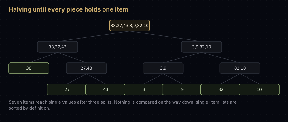
Nothing has been sorted yet. Splitting a list never compares anything: it just produces smaller lists. Notice how few levels this takes: seven items reach single values after three splits, because each split halves the size. A thousand items would take ten.
Merging back up
Now the tree unwinds, and every merge combines two sorted lists into one longer sorted list. The interesting one is the last: merging [27, 38, 43] with [3, 9, 10, 82]. Follow the two fingers.
27against3— take3. The right finger moves.27against9— take9.27against10— take10.27against82— take27. Now the left finger moves.38against82— take38.43against82— take43. The left list is now empty.- Nothing left to compare. Copy the rest of the right list,
[82], straight across.
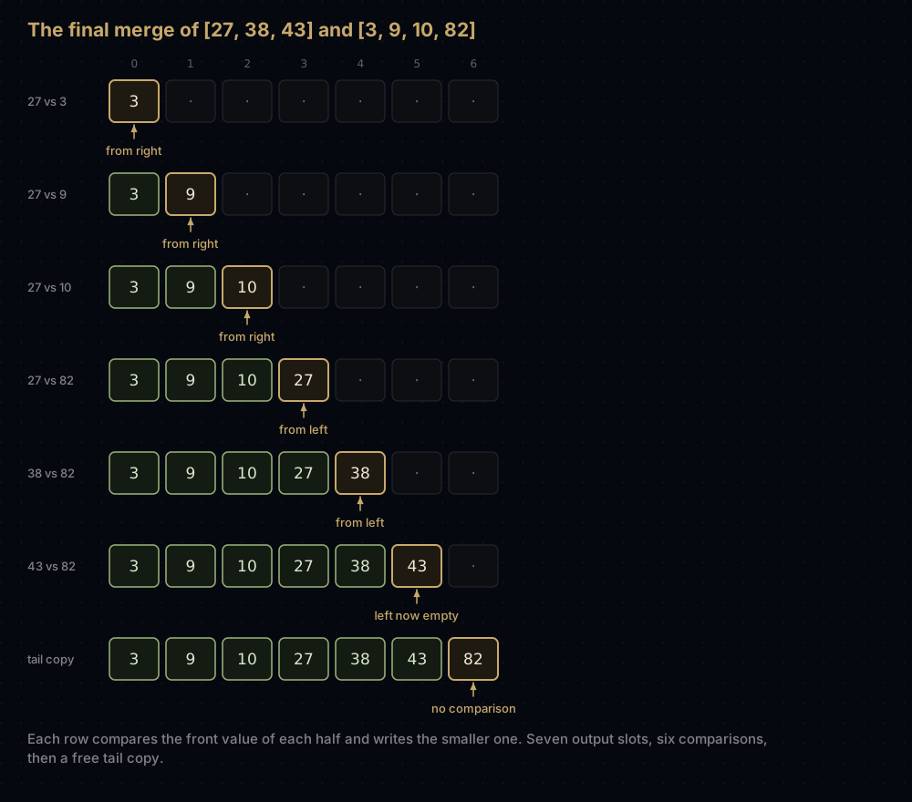
Seven output slots filled with six comparisons and one free copy. That is the pattern every merge follows: at most one comparison per output slot, often fewer thanks to the tail copy.
Every level, in order
Stack the merges by level and the shape of the algorithm appears:
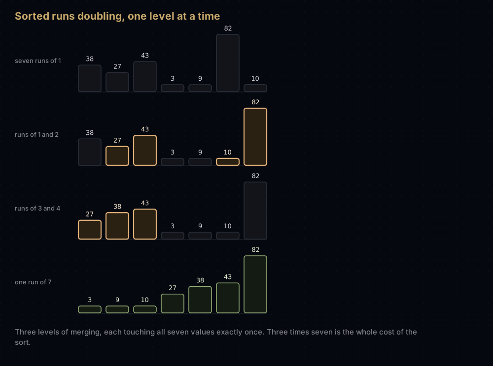
Level by level the sorted runs double in length: seven runs of one, then runs of one, two, two and two, then runs of three and four, then a single run of seven. Three levels of merging, and each level touches all seven items once. Three times seven is the entire cost of the sort: the counting argument in miniature, which the complexity section below simply rewrites for n.
The code
Start with the merge, since it carries the algorithm.
def merge(left: list[int], right: list[int]) -> list[int]:
    """Combine two already-sorted lists into one sorted list.

    Walks both lists with one index each, always taking the smaller of the two
    front values, so every element is looked at exactly once.
    """
    merged: list[int] = []
    left_index = right_index = 0

    while left_index < len(left) and right_index < len(right):
        # <= not < : on a tie the left list wins, and the left list holds the
        # values that came earlier in the original input. That is stability.
        if left[left_index] <= right[right_index]:
            merged.append(left[left_index])
            left_index += 1
        else:
            merged.append(right[right_index])
            right_index += 1

    # One list is now empty. Whatever remains in the other is already sorted and
    # already larger than everything placed so far, so it is copied across whole.
    merged.extend(left[left_index:])
    merged.extend(right[right_index:])
    return merged


print(merge([27, 38, 43], [3, 9, 10, 82]))
print(merge([1, 2], []))
print(merge([], []))[3, 9, 10, 27, 38, 43, 82]
[1, 2]
[]The sort itself is then five lines, and reads exactly like the three-step description.
def merge_sort(items: list[int]) -> list[int]:
    """Sort a list ascending by splitting it in half, sorting each half, then
    merging the two sorted halves back together.

    Returns a new list; the caller's list is left untouched.
    """
    # A list of zero or one item is already sorted. This is the base case, and
    # the only branch that does not recurse.
    if len(items) <= 1:
        return list(items)

    middle = len(items) // 2
    left = merge_sort(items[:middle])
    right = merge_sort(items[middle:])
    return merge(left, right)


print(merge_sort([38, 27, 43, 3, 9, 82, 10]))
print(merge_sort([]))
print(merge_sort([5]))
print(merge_sort([2, 1]))
print(merge_sort([4, 4, 4, 1]))[3, 9, 10, 27, 38, 43, 82]
[]
[5]
[1, 2]
[1, 4, 4, 4]To check the walkthrough above was not wishful thinking, print every merge as it happens, indented by how deep in the recursion it is.
def merge_sort_traced(items: list[int], depth: int = 0) -> list[int]:
    """Merge sort that prints every merge, indented by recursion depth."""
    if len(items) <= 1:
        return list(items)

    middle = len(items) // 2
    left = merge_sort_traced(items[:middle], depth + 1)
    right = merge_sort_traced(items[middle:], depth + 1)
    result = merge(left, right)
    print(f"{'    ' * depth}merge {left} + {right} -> {result}")
    return result


merge_sort_traced([38, 27, 43, 3, 9, 82, 10]) merge [27] + [43] -> [27, 43]
merge [38] + [27, 43] -> [27, 38, 43]
merge [3] + [9] -> [3, 9]
merge [82] + [10] -> [10, 82]
merge [3, 9] + [10, 82] -> [3, 9, 10, 82]
merge [27, 38, 43] + [3, 9, 10, 82] -> [3, 9, 10, 27, 38, 43, 82]Six merges for seven items, and the deepest ones finish first. The left half is completely sorted before the right half is even looked at, because merge_sort(items[:middle]) has to return before the next line runs.
How the code maps to the idea
The base case is len(items) <= 1, not len(items) == 0. This is the difference between working code and an infinite loop. A one-item list has middle == 0, so items[:0] is empty and items[0:] is the same one-item list you started with: the recursion would call itself forever with unchanged input. Checking for one item is what actually terminates the algorithm.
The split is items[:middle] and items[middle:], sharing the same index. Every element lands in exactly one half, nothing is dropped or duplicated. With an odd length the right half gets the extra item, which does not matter at all: merge sort does not care whether the halves are equal, only that both are smaller than the original.
The recursion depth is not a problem. Each call halves the list, so the deepest chain is ⌈log₂ n⌉ frames. Python's default recursion limit is 1000, and merge sort would need a list of 2¹⁰⁰⁰ items to reach it, unlike a naive recursive factorial, which hits that limit at around n = 1000.
The <= in the merge is what makes the sort stable. When the two front values compare equal, the left list wins the tie. The left list is the earlier half of the original input, so equal items come out in their original relative order. Sort a list of records by score with this and the ties stay in input order:
from typing import Any, Callable


def merge_sort_by(items: list[Any], key: Callable[[Any], Any]) -> list[Any]:
    """Merge sort ordering by key(item), keeping equal keys in input order."""
    if len(items) <= 1:
        return list(items)

    middle = len(items) // 2
    left = merge_sort_by(items[:middle], key)
    right = merge_sort_by(items[middle:], key)

    merged: list[Any] = []
    left_index = right_index = 0
    while left_index < len(left) and right_index < len(right):
        if key(left[left_index]) <= key(right[right_index]):
            merged.append(left[left_index])
            left_index += 1
        else:
            merged.append(right[right_index])
            right_index += 1
    merged.extend(left[left_index:])
    merged.extend(right[right_index:])
    return merged


scores = [("ana", 90), ("bo", 75), ("cy", 90), ("dee", 75), ("eli", 90)]
for name, score in merge_sort_by(scores, key=lambda row: row[1]):
print(f"{name:<4} {score}")bo 75
dee 75
ana 90
cy 90
eli 90Both 75s and all three 90s kept their input order. Change that one <= to < and the sort is still correct but no longer stable: the same input comes out as dee, bo, eli, cy, ana, with every tie group reversed. Stability is what lets you sort by name and then by score and end up with names ordered inside each score.
Top-down and bottom-up
The version above is top-down: recurse to the bottom, then merge on the way back up. There is an equivalent bottom-up version that skips the recursion entirely. Treat the list as n sorted runs of length 1, merge neighbouring runs into runs of length 2, then 4, then 8, until one run covers everything.
def merge_sort_bottom_up(items: list[int]) -> list[int]:
    """Iterative merge sort: merge runs of width 1, then 2, then 4, and so on."""
    values = list(items)
    n = len(values)

    width = 1
    while width < n:
        for start in range(0, n, 2 * width):
            middle = min(start + width, n)
            end = min(start + 2 * width, n)
            # On an odd-sized list the final chunk can give middle == end, which
            # merges against an empty right half. Harmless, so no special case.
            values[start:end] = merge(values[start:middle], values[middle:end])
        width *= 2

    return values


print(merge_sort_bottom_up([38, 27, 43, 3, 9, 82, 10]))
print(merge_sort_bottom_up([5, 4, 3, 2, 1, 0]))
print(merge_sort_bottom_up([]))[3, 9, 10, 27, 38, 43, 82]
[0, 1, 2, 3, 4, 5]
[]Same result, same O(n log n), the same total work arranged differently, on a list whose length is not a power of two the two versions do not even merge the same pairs. The while width < n loop runs ⌈log₂ n⌉ times and each pass touches every element, which is the complexity argument made visible as two loops. Bottom-up is what you write when recursion is expensive or unavailable. It is the shape the Linux kernel uses in lib/list_sort.c for sorting linked lists.
Complexity
Every bound merge sort has comes from two facts, and they are worth writing separately.
Fact one: there are ⌈log₂ n⌉ levels. The list is halved on the way down, so the sizes go n, n/2, n/4, n/8 and so on. Ask how many halvings it takes to get from n to 1 and you are asking what power of 2 reaches n. That is the definition of a base-2 logarithm. A million items take 20 levels, because 2²⁰ is a little over a million. A billion items take 30.
Fact two: each level costs O(n). At any level the sublists are disjoint pieces of the original list, and together they cover all n elements. Merging two lists holding m items between them costs at most m − 1 comparisons and exactly m writes, so summing across one level gives at most n comparisons and exactly n writes: regardless of how many pieces that level is cut into.
Multiply: log₂ n levels times O(n) per level is O(n log n). As a recurrence, T(n) = 2T(n/2) + O(n), which resolves to the same thing.
The crucial point is that neither fact depends on the data. The number of levels is fixed by the length of the list, and every level looks at every element whatever order it is in. So the best case, average case and worst case are all Θ(n log n). Merge sort cannot be given a bad day.
It can be given a slightly cheaper one. When one half is entirely smaller than the other, the merge exhausts that half and copies the rest for free, using only m/2 comparisons instead of m − 1. That halves the comparison count, but not the growth rate. Count it and see:
def merge_sort_counted(items: list[int]) -> tuple[list[int], int]:
    """Merge sort that also reports how many element comparisons it made."""
    comparisons = 0

    def sort(values: list[int]) -> list[int]:
        nonlocal comparisons
        if len(values) <= 1:
            return list(values)

        middle = len(values) // 2
        left = sort(values[:middle])
        right = sort(values[middle:])

        merged: list[int] = []
        left_index = right_index = 0
        while left_index < len(left) and right_index < len(right):
            comparisons += 1
            if left[left_index] <= right[right_index]:
                merged.append(left[left_index])
                left_index += 1
            else:
                merged.append(right[right_index])
                right_index += 1
        merged.extend(left[left_index:])
        merged.extend(right[right_index:])
        return merged

    return sort(items), comparisons


_, small = merge_sort_counted([38, 27, 43, 3, 9, 82, 10])
print(f"the 7-item worked example: {small} comparisons")

size = 1024
cases = [
    ("already sorted", list(range(size))),
    ("shuffled      ", [(index * 401) % size for index in range(size)]),
    ("reversed      ", list(range(size - 1, -1, -1))),
]
for label, data in cases:
    result, comparisons = merge_sort_counted(data)
    assert result == sorted(data)
    print(f"{label}  {comparisons:>6} comparisons")

print(f"n log2 n        {size * 10:>6}")
print(f"n squared / 2 {size * size // 2:>6}")the 7-item worked example: 13 comparisons
already sorted 5120 comparisons
shuffled 9134 comparisons
reversed 5120 comparisons
n log2 n 10240
n squared / 2 524288Three completely different inputs, and the counts sit between 5,120 and 9,134: a factor of 1.8 apart, with the theoretical n log₂ n of 10,240 just above the top. A quadratic sort on the same 1,024 items would need around half a million comparisons on average. Note that reversed input is a cheap case here, not an expensive one: every merge empties its right half first and copies the left half across untouched.
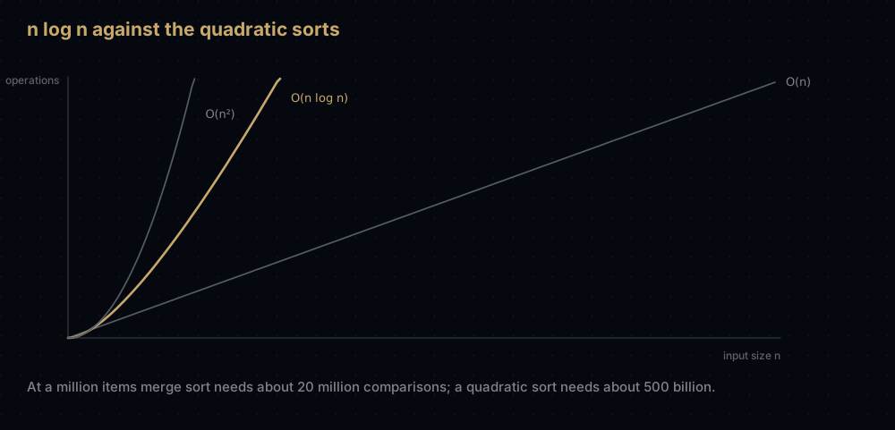
Space: O(n), and this is the real cost. Each merge builds a brand-new list rather than rearranging one in place. The peak is the top-level merge: it fills an output of n while still holding the two sorted halves that feed it, n/2 each, and the half-sized slices left alive further down the chain add n/2 + n/4 + … on top of that. The total is a small constant times n, so live memory is O(n), and the ⌈log₂ n⌉ recursion frames, the other thing the sort consumes, vanish beside it. What grows as O(n log n) is not the number of lists allocated: that is a fixed handful per call across 2n − 1 calls, so O(n). It is the number of elements copied, because every one of the log n levels copies all n of them, and in Python that copying and allocation is a real share of the runtime. Serious implementations allocate one scratch buffer up front and reuse it for every merge; CPython's Timsort keeps a temporary buffer no larger than half the list.
Why not merge in place? Because it is genuinely hard. In-place merge algorithms exist — block merge sort and its relatives — but they need rotations and internal buffers that turn a tight linear merge into something with large constants, and the code is many times longer. In practice nobody ships them for arrays. If you need O(n log n) with O(1) space, use heap sort. The one exception is linked lists: merging two sorted linked lists only rewires pointers and allocates no nodes, so a bottom-up linked-list merge sort really is O(1) extra space: the recursive top-down version still pays for its ⌈log₂ n⌉ stack frames. That is why merge sort is the standard way to sort a linked list.
| Items | Merge sort, about n log₂ n | Quadratic sort, about n² / 2 |
|---|---|---|
| 1,000 | 10,000 | 500,000 |
| 100,000 | 1,700,000 | 5,000,000,000 |
| 1,000,000 | 20,000,000 | 500,000,000,000 |
At a million items the gap is 25,000-fold, for Python-level code, the difference between seconds and days.
When to use it, and when not to
Use it when you need a worst-case guarantee. Quick sort's average case is faster, but its worst case is O(n²), and on inputs an attacker chooses it can be triggered deliberately. If a slow sort means a missed deadline or a denial-of-service, merge sort's flat guarantee is worth the memory.
Use it when you need stability. Sorting a table by one column and then another only works if the second sort preserves the first's ordering. Merge sort is stable for free; quick sort and heap sort are not.
Use it when the data does not fit in memory. This is merge sort's uncontested territory, covered below.
Use it for linked lists. No random access is needed — you only ever look at the front of each list — so merge sort runs at full speed on a structure where quick sort and heap sort are hopeless.
Do not use it when memory is tight, when the data fits in cache and raw speed is everything (quick sort's in-place partitioning has much better locality), or when n is small. Below roughly 16 to 32 elements the recursion overhead outweighs everything and insertion sort wins outright, which is why real implementations switch to insertion sort for small chunks.
And in day-to-day Python, do not write it at all. Call sorted(items) or items.sort(). Timsort is written in C, is stable, is O(n log n) worst case, and will beat any Python-level sort you write by a factor of a hundred or more.
Where it shows up in the real world
Timsort, and therefore sorted(). Timsort is a natural merge sort: it scans for runs that are already ascending or descending, extends short runs to a minimum length with binary insertion sort, and then merges those runs under an invariant on the lengths of the runs still waiting, which keeps every merge roughly balanced. Everything after the run detection is the merge you wrote above, plus "galloping": using binary search to skip long stretches when one run is consistently winning. It is the sort behind Python's sorted() and list.sort(), and behind Java's Arrays.sort for object arrays. Rust's stable slice::sort is a relative rather than the same algorithm: also a stable, run-detecting merge sort, but with its own merge strategy. Merge sort is not a stepping stone to any of them; it is them, with the run detection bolted on. The full story is in Timsort.
External sorting — files larger than memory. Suppose you must sort a 200 GB log file on a machine with 8 GB of RAM. Read the file in 4 GB chunks, sort each chunk in memory, write it back out as a temporary sorted file. That gives you fifty sorted runs. Now merge all fifty at once: keep a small read buffer from each file, repeatedly take the smallest of the fifty front values, and stream the result to the output. Memory holds fifty buffers, never the data. Every read and write is sequential, which is what disks and object stores are fastest at.
That is exactly what GNU coreutils sort does when its input exceeds its buffer, and what PostgreSQL does when an ORDER BY exceeds work_mem: EXPLAIN ANALYZE reports the sort method as external merge with the temporary disk usage. Merge sort is the only classic comparison sort that adapts to this, because the merge step never needs random access: it reads each input strictly front to back and writes its output strictly front to back.
Python ships the merge step for you, and it is lazy, so it works on file handles just as well as lists:
import heapq

runs = [[3, 9, 10, 82], [27, 38, 43], [1, 60]]
print(list(heapq.merge(*runs)))[1, 3, 9, 10, 27, 38, 43, 60, 82]heapq.merge takes any number of sorted iterables and yields their merge, using a heap to find the smallest front value among k inputs in O(log k) time. Swap those lists for open files and you have written the merge phase of an external sort.
Parallel and distributed sorting. The two halves are completely independent, so they can be sorted on different cores or different machines with no coordination at all. The sort-merge step in MapReduce-style systems is built on exactly this property.
Common mistakes
A base case of len(items) == 0. A one-item list then splits into an empty half and itself, and the recursion never ends. Test with a single-element list.
Forgetting the tail copy. Drop the two merged.extend(...) lines and the merge loop ends the moment either list runs out, silently discarding the remainder. The result is sorted but short, which is exactly the kind of bug that passes a casual eyeball check.
Splitting with items[middle + 1:]. That skips the element at middle. It is a habit borrowed from binary search, where the middle element has already been examined; here it has not.
Using < instead of <=. Still sorts, silently loses stability. It only shows up later, when someone relies on a previous sort surviving this one.
Merging lists that are not sorted yet. Both recursive calls must complete before the merge. The whole correctness argument rests on both inputs being sorted, so a merge placed before the recursion produces garbage.
Allocating a fresh list per merge. Fine for learning, wasteful in production. If a hand-written merge sort profiles slower than you expected, the allocator is usually the reason.
Practice
- Merge two sorted lists into one without using
sorted(), then check your function againstheapq.merge. - Add a cutoff so that sublists of 16 or fewer items are sorted with insertion sort instead of recursing further, and count how many merge calls this removes.
- Count inversions — pairs where a larger value sits before a smaller one — by adding a counter to the merge, incremented by the number of items left in the left half whenever you take from the right.
- Write a natural merge sort: scan the input once for runs that are already ascending, then merge those runs instead of starting from single elements. Compare its merge count to plain merge sort on nearly-sorted input.
- Implement merge sort for a singly linked list, splitting with a slow and fast pointer and merging by rewiring
nextpointers so that no new nodes are allocated.
Summary
Merge sort is the algorithm to reach for when you need a guarantee rather than an average. Its cost is fixed by the structure of the recursion, not by the data: ⌈log₂ n⌉ levels of halving, O(n) work to merge each level, therefore Θ(n log n) on every input that exists. It pays for that with O(n) scratch memory, and buys back stability and the ability to sort data that never fits in memory at once.
| Difficulty | Medium |
| Best case | O(n log n) — the level structure is fixed by n, not by the data |
| Average case | O(n log n) |
| Worst case | O(n log n) — no input makes it slower |
| Space | O(n) — the merge writes into a new buffer; O(1) for a bottom-up linked-list version |
| Stable | Yes — <= in the merge lets the earlier half win every tie |
| In place | No — in-place merging exists but is impractical for arrays |
| Adaptive | No on its own; Timsort adds run detection to make it adaptive |
| Data structure | List / array, and linked lists especially well |
| Use it when | You need worst-case O(n log n), stability, or data larger than memory |
| Avoid it when | Memory is tight, n is tiny, or raw in-cache speed matters most |
| Real-world use | Timsort in Python, Java and Rust; GNU sort and database external sorts |
| Python equivalent | sorted(items) / items.sort(); heapq.merge for the merge step |
The next algorithm to learn is quick sort, which attacks the same problem from the opposite direction: it does the hard work before recursing rather than after, sorts in place, and trades merge sort's guarantee for better average speed.
Keep reading
- Quick Sort in Python — the other O(n log n) divide-and-conquer sort, and why it usually wins despite a worse worst case.
- Heap Sort in Python — O(n log n) with O(1) space, the option when merge sort's buffer is unaffordable.
- Timsort — what
sorted()actually runs: merge sort plus run detection and galloping. - Recursion and Backtracking — the mental model for base cases and recursive calls used throughout this post.
- Big O Notation — the counting arguments behind O(n log n) and why the constants were dropped.


