Heap sort is the only common sorting algorithm that gives you two guarantees at once: O(n log n) on every input without exception, and a fixed amount of extra memory however long the list is. Merge sort matches the time bound but needs a scratch array of n elements. Quick sort sorts in place as well, apart from the O(log n) call stack its recursion needs, but collapses to O(n²) on inputs that a careless pivot choice — or a deliberate attacker — can hand it. Heap sort does neither.
It pays for that with a trick worth learning on its own: it builds a binary tree inside the array you were already given, with no nodes and no pointers. Position in the array is the tree structure. Once you see that, half the algorithm becomes obvious.
The caveat belongs up front. On ordinary random data heap sort is usually two to three times slower than quick sort, and the reason is the memory access pattern rather than the big-O. So it rarely runs on its own. It runs as the safety net underneath quick sort in C++'s std::sort, and as the sort of choice inside the Linux kernel, where a worst case that cannot be triggered beats being fastest on average.
The idea
An array is already a tree
A binary max-heap is a binary tree with exactly two rules:
- Shape. Every level is completely full except possibly the last, which fills left to right with no gaps. Such a tree is called complete.
- Order. Every parent is greater than or equal to both of its children.
Rule 2 is weaker than it looks: it says nothing about left child versus right child, or about cousins. The one certainty is that the largest value sits at the root, because every node is beaten by its parent and the chain of parents ends there.
The shape rule is what lets the tree live in a flat array. Number the nodes level by level from 0; with no gaps, the arithmetic works out exactly:
- the left child of index
iis at2 * i + 1 - the right child of index
iis at2 * i + 2 - the parent of index
iis at(i - 1) // 2
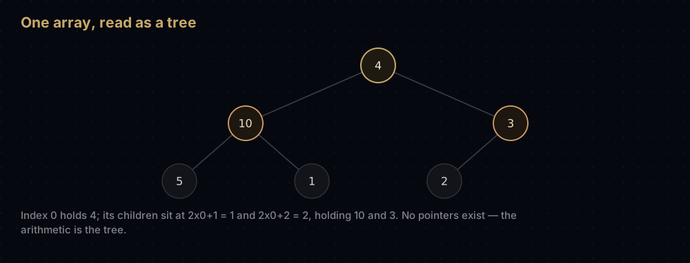
The tree is an interpretation of the array, recomputed on demand: no pointers, no node objects. Any list of n items is a complete binary tree read this way; the only question is whether it obeys the order rule.
Index i has a left child only if 2 * i + 1 is inside the array, which fails from n // 2 onwards. So the whole second half is leaves, and a leaf is already a valid one-node heap: a fact the complexity argument leans on hard.
Sift down: the one operation
Everything in heap sort is built from one move, sift down (also called heapify or percolate down). Take a node whose two subtrees are already valid max-heaps but whose own value may be too small. Compare it with the larger of its two children; if that child is bigger, swap, then repeat from the position the value moved into. Stop when both children lose, or you run off the bottom.
Each step costs one swap and one level of descent, so a sift down from a node of height h costs at most h swaps and 2h comparisons: one comparison to pick the larger child, one to test it against the parent. A complete tree of n nodes has height floor(log2(n)), so no sift down ever costs more than about log₂ n steps.
Two phases
Phase 1 — build the heap. Sift down every non-leaf index, walking backwards from n // 2 - 1 to 0. Backwards is not a stylistic choice: sift down assumes the subtrees below a node are already heaps, and decreasing index order is what makes that true.
Phase 2 — extract, n − 1 times. The root holds the maximum, and you know where the maximum belongs: the last slot. Swap them, then shrink the heap by one so the finished slot is out of reach. The root now holds whatever was at the end, breaking the order rule at exactly one node, so sift it down and repeat. The sorted region grows leftwards from the right-hand end, and the array comes out ascending.
Watching it work
Take [4, 10, 3, 5, 1, 2]. Six items, so the last non-leaf is at index 6 // 2 - 1 = 2, and indices 3, 4, 5 are leaves.
i = 2 (value 3). Its only child is index 5, holding 2, which does not beat 3. Nothing moves.
i = 1 (value 10). Children are 5 and 1. The larger, 5, does not beat 10. Nothing moves.
i = 0 (value 4). Children are 10 and 3. 10 beats 4, so they swap: [10, 4, 3, 5, 1, 2]. The 4 now sits at index 1 with children 5 and 1; 5 beats 4, so they swap: [10, 5, 3, 4, 1, 2]. The 4 lands on index 3, a leaf. Stop.
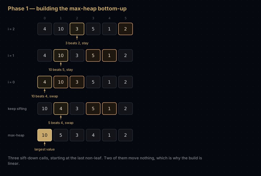
Two of the three sift downs did no work at all. That is not luck — it is the shape of the O(n) argument below.
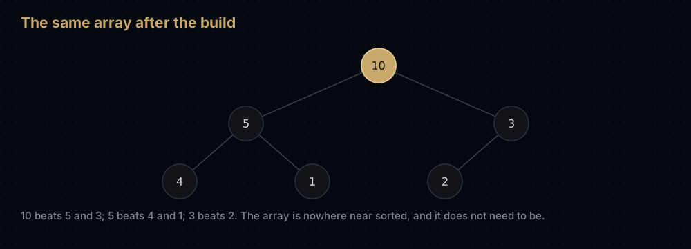
Check the order rule against the tree: 10 beats 5 and 3; 5 beats 4 and 1; 3 beats 2. The array is nowhere near sorted — 3 sits before 4 — and it does not need to be. A heap is a much weaker promise than a sorted list, which is precisely why it is cheap to build.
Now extract. Swap the root 10 with index 5: [2, 5, 3, 4, 1, 10], and index 5 is finished forever. The heap is the first five slots, with 2 at its root. Sift it down: children 5 and 3, so swap with 5 → [5, 2, 3, 4, 1]; the 2 sits at index 1 with children 4 and 1, so swap with 4 → [5, 4, 3, 2, 1]. The array reads [5, 4, 3, 2, 1, 10].
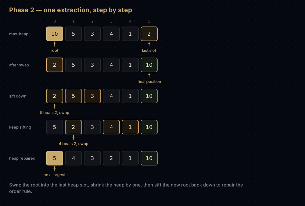
Four more rounds do the same on a heap one slot shorter each time: 5 moves to index 4 and 4 rises to the root, then 4 moves to index 3, then 3 to index 2, then 2 to index 1 — leaving [1, 2, 3, 4, 5, 10]. The traced run further down prints every one of those states.
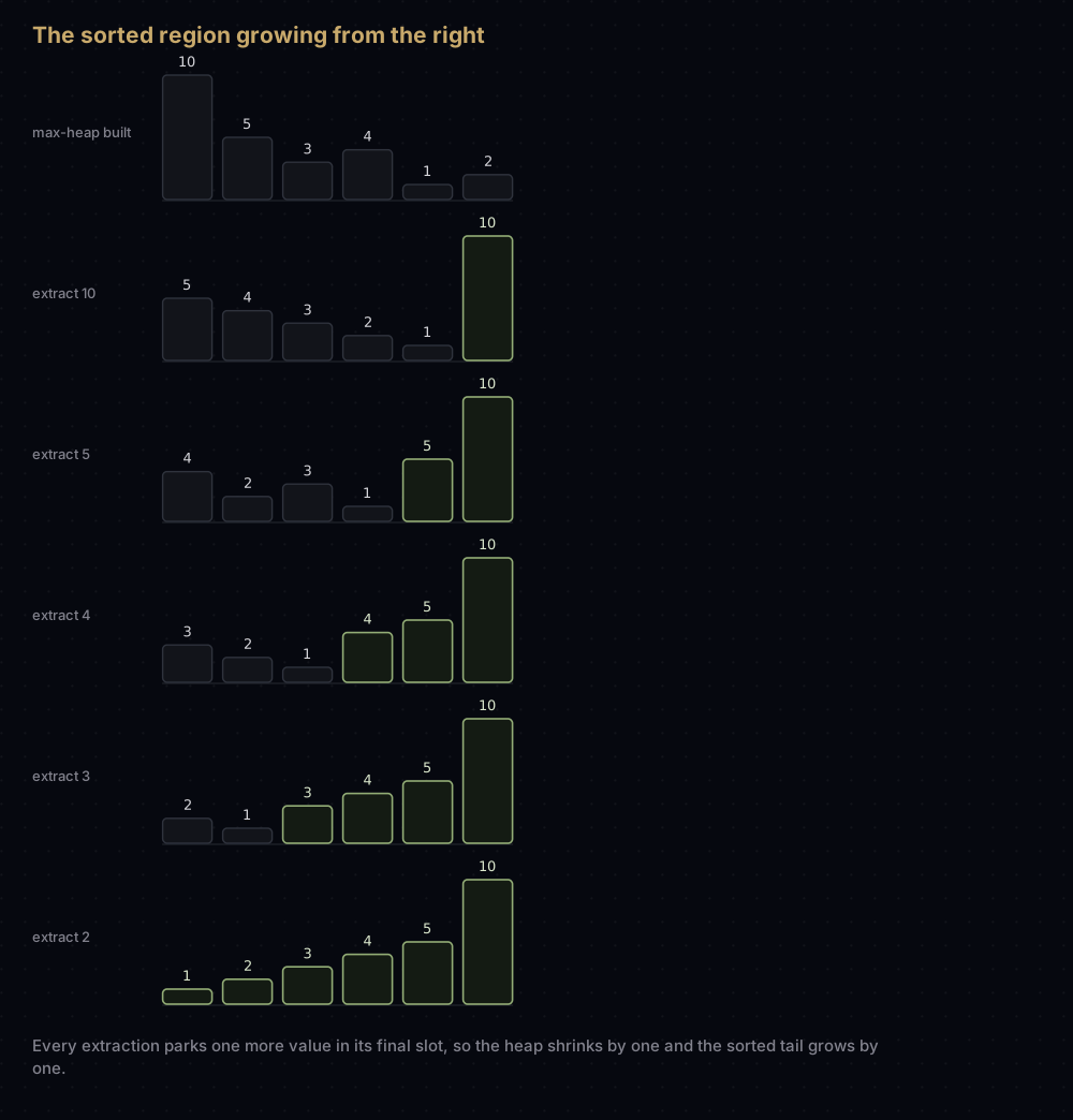
Five extractions, and nothing was ever copied out of the array.
The code
def sift_down(values: list[int], start: int, end: int) -> None:
    """Push the value at `start` down until both its children are smaller.

    Only indices below `end` belong to the heap. Anything from `end` onwards is
    already in its final sorted position and must not be touched.
    """
    root = start
    while True:
        left = 2 * root + 1
        right = left + 1
        largest = root

        if left < end and values[left] > values[largest]:
            largest = left
        if right < end and values[right] > values[largest]:
            largest = right
        if largest == root:
            # Both children lose, so the order rule holds from here down.
            return

        values[root], values[largest] = values[largest], values[root]
        root = largest


def heap_sort(values: list[int]) -> None:
    """Sort `values` ascending, in place, using O(1) extra memory."""
    n = len(values)

    # Phase 1: build a max-heap bottom-up. Indices n // 2 and above are leaves,
    # and a leaf is already a valid one-node heap, so they need no work.
    for start in range(n // 2 - 1, -1, -1):
        sift_down(values, start, n)

    # Phase 2: the maximum is always at index 0. Swap it to the end of the
    # shrinking heap, then repair the single node that broke.
    for end in range(n - 1, 0, -1):
        values[0], values[end] = values[end], values[0]
        sift_down(values, 0, end)


data = [4, 10, 3, 5, 1, 2]
heap_sort(data)
print(data)

for case in ([], [7], [2, 2, 2], [5, 4, 3, 2, 1]):
    heap_sort(case)
print(case)[1, 2, 3, 4, 5, 10]
[]
[7]
[2, 2, 2]
[1, 2, 3, 4, 5]Two short functions, no recursion, no allocation. The standard library ships the heap half of this as heapq, which keeps a min-heap in a plain list using the same O(n) bottom-up build:
import heapq

values = [4, 10, 3, 5, 1, 2]
heapq.heapify(values)  # the same bottom-up build, but for a min-heap
print(values)
print([heapq.heappop(values) for _ in range(6)])[1, 4, 2, 5, 10, 3]
[1, 2, 3, 4, 5, 10]Popping every element gives a sorted list — heap sort in two lines — but it costs a second list, throwing away the property that makes heap sort worth knowing. There is no in-place heap sort in the standard library, and for real work you want sorted() anyway.
How the code maps to the idea
The end parameter is the entire in-place trick. sift_down never looks at an index at or past end. Phase 2 shrinks end by one each round, so the growing sorted tail and the shrinking heap share one array with no boundary marker and no copy. One integer separates finished from unfinished.
range(n // 2 - 1, -1, -1) is the backwards build: start at the last non-leaf and finish at 0 inclusive, since the middle -1 is the stop value that range excludes. By the time the loop reaches index i, everything below it is already a heap. range(n - 1, 0, -1) then stops at 1, because a one-element heap has nothing left to swap with.
Two comparisons per level, not one. The code picks the larger child first, then decides whether to move. Comparing the parent against only the left child is the classic broken version: it leaves a bigger right child sitting under a smaller parent.
largest == root is the early exit, and the loop is iterative rather than recursive. A recursive sift down reads better but burns O(log n) stack frames, quietly breaking the O(1) space claim.
Edge cases fall out of the arithmetic. For an empty or one-element list n // 2 - 1 is −1 or less, range(-1, -1, -1) is empty, and both loops skip.
Here is the same algorithm printing the array after every sift down, so you can check the walkthrough line by line:
def heap_sort_traced(values: list[int]) -> None:
    """Heap sort that prints the array after every sift down."""
    n = len(values)
    print(f"{'start':<16}{values}")

    for start in range(n // 2 - 1, -1, -1):
        sift_down(values, start, n)
        print(f"{'build i=' + str(start):<16}{values}")

    for end in range(n - 1, 0, -1):
        values[0], values[end] = values[end], values[0]
        sift_down(values, 0, end)
        print(f"{'heap size ' + str(end):<16}{values}")


heap_sort_traced([4, 10, 3, 5, 1, 2])start [4, 10, 3, 5, 1, 2]
build i=2 [4, 10, 3, 5, 1, 2]
build i=1 [4, 10, 3, 5, 1, 2]
build i=0 [10, 5, 3, 4, 1, 2]
heap size 5 [5, 4, 3, 2, 1, 10]
heap size 4 [4, 2, 3, 1, 5, 10]
heap size 3 [3, 2, 1, 4, 5, 10]
heap size 2 [2, 1, 3, 4, 5, 10]
heap size 1 [1, 2, 3, 4, 5, 10]Heap sort is not stable
A sort is stable if items that compare equal come out in the order they went in, which matters whenever you sort by one field after another. Heap sort is not stable, and the reason is structural rather than fixable: the root-to-end swap flings two values across the whole array, past every equal value in between.
def heap_sort_by(values: list, key) -> None:
    """Heap sort ordered by key(item) alone, so equal keys are genuinely tied."""
    n = len(values)

    def sift(start: int, end: int) -> None:
        root = start
        while True:
            left, right, largest = 2 * root + 1, 2 * root + 2, root
            if left < end and key(values[left]) > key(values[largest]):
                largest = left
            if right < end and key(values[right]) > key(values[largest]):
                largest = right
            if largest == root:
                return
            values[root], values[largest] = values[largest], values[root]
            root = largest

    for start in range(n // 2 - 1, -1, -1):
        sift(start, n)
    for end in range(n - 1, 0, -1):
        values[0], values[end] = values[end], values[0]
        sift(0, end)


by_score = [(1, "ana"), (1, "ben"), (0, "cal")]
heap_sort_by(by_score, key=lambda pair: pair[0])
print("heap sort:", by_score)
print("sorted():", sorted([(1, "ana"), (1, "ben"), (0, "cal")], key=lambda pair: pair[0]))heap sort: [(0, 'cal'), (1, 'ben'), (1, 'ana')]
sorted(): [(0, 'cal'), (1, 'ana'), (1, 'ben')]Ana went in before Ben and came out after him. sorted(), which is stable, keeps them in input order. If stability matters, merge sort is the right tool.
Complexity
Building the heap is O(n), not O(n log n)
The obvious argument gives the wrong answer: there are about n/2 non-leaf nodes, each sift down costs up to log₂ n, therefore the build is O(n log n). That bound is true, just not tight, because it charges every node the price of the root, and only one node is the root.
Count by height instead of by index. A node's height is the number of edges on the longest path from it down to a leaf. Then:
- a sift down from a node of height h costs at most h swaps;
- at most n / 2^(h+1) nodes sit at height h, rounded up. Leaves are about half the array, height-1 nodes about a quarter, height-2 nodes an eighth, and so on.
So the total build work is at most the sum, over every height h from 0 to log₂ n, of (n / 2^(h+1)) × h. Pull n/2 out front and you are left with n/2 times the sum of h / 2^h: a series that converges to exactly 2. The build therefore costs at most n swaps.
Read as an English sentence it stops being magic: the nodes that can move a long way are rare, and the nodes that are plentiful can barely move at all. Half the array is leaves that cannot move. The single node that can fall the full log₂ n levels is the root.
Here is that sum for a perfect heap with 1,048,575 nodes, worked out exactly:
def build_bound(levels: int) -> None:
    """Print the worst-case swap budget for building a perfect max-heap."""
    n = 2 ** levels - 1
    total = 0
    print(f"perfect max-heap, n = {n:,} nodes")
    print(f"{'height':>7}{'nodes':>12}{'swaps each':>12}{'subtotal':>13}")
    for height in range(levels):
        nodes = 2 ** (levels - 1 - height)
        total += nodes * height
        if height <= 4:
            print(f"{height:>7}{nodes:>12,}{height:>12}{nodes * height:>13,}")
    print(f"{'...':>7}{'...':>12}{'...':>12}{'...':>13}")
    print(f"total swaps to build the heap: {total:,}")
    print(f"that is {total / n:.5f} x n -- linear, not n log n")


build_bound(20)perfect max-heap, n = 1,048,575 nodes
height nodes swaps each subtotal
0 524,288 0 0
1 262,144 1 262,144
2 131,072 2 262,144
3 65,536 3 196,608
4 32,768 4 131,072
... ... ... ...
total swaps to build the heap: 1,048,555
that is 0.99998 x n -- linear, not n log n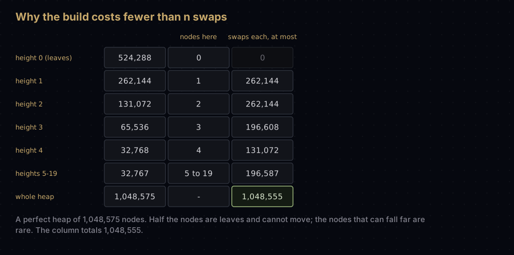
A million-node heap costs under a million swaps to build, and that is a hard bound rather than an average.
The extraction phase is Θ(n log n)
Phase 2 runs n − 1 rounds. Round k sifts one value down from the root of a heap of size k, costing at most log₂ k swaps. Summing log₂ k for k from 1 to n gives log₂(n!), which Stirling's approximation puts at n log₂ n − 1.44n. Upper bound: O(n log n).
The lower bound is why heap sort has no good case. The value promoted to the root each round was, one instant earlier, in the last slot of the heap: a leaf, and a leaf is smaller than every one of its roughly log₂ n ancestors. Small values at the top sink, so nearly every round pays close to full depth. That holds whatever the input looks like: on distinct keys heap sort's best case is Θ(n log n) as well, and an already-sorted array costs about as many comparisons as a shuffled one. Unlike insertion sort or Timsort, no arrangement lets it finish early.
The one degenerate exception is an array where every key is equal. Then values[left] > values[largest] is false immediately, every sift down returns after two comparisons, and the sort is O(n). A curiosity, not a feature.
Measured on real arrays, with a deterministic shuffle so the numbers reproduce:
import math


def shuffled(n: int) -> list[int]:
    """A deterministic shuffle, so these counts are the same on every machine."""
    values = list(range(n))
    state = 12345
    for index in range(n - 1, 0, -1):
        state = (1103515245 * state + 12345) % (1 << 31)
        other = state % (index + 1)
        values[index], values[other] = values[other], values[index]
    return values


def heap_sort_counted(values: list[int]) -> tuple[int, int]:
    """Sort in place, returning (build-phase swaps, extract-phase swaps)."""
    n = len(values)
    build = extract = 0

    def sift(start: int, end: int) -> int:
        moves = 0
        root = start
        while True:
            left, right, largest = 2 * root + 1, 2 * root + 2, root
            if left < end and values[left] > values[largest]:
                largest = left
            if right < end and values[right] > values[largest]:
                largest = right
            if largest == root:
                return moves
            values[root], values[largest] = values[largest], values[root]
            root = largest
            moves += 1

    for start in range(n // 2 - 1, -1, -1):
        build += sift(start, n)
    for end in range(n - 1, 0, -1):
        values[0], values[end] = values[end], values[0]
        extract += 1 + sift(0, end)
    return build, extract


for size in (1_000, 10_000, 100_000):
    items = shuffled(size)
    build, extract = heap_sort_counted(items)
    assert items == sorted(items)
    print(f"n = {size:>7,}   build {build:>8,} swaps = {build / size:.2f} n"
f" extract {extract:>9,} swaps = {extract / (size * math.log2(size)):.2f} n log2 n")n = 1,000 build 764 swaps = 0.76 n extract 8,360 swaps = 0.84 n log2 n
n = 10,000 build 7,788 swaps = 0.78 n extract 116,965 swaps = 0.88 n log2 n
n = 100,000 build 78,857 swaps = 0.79 n extract 1,502,845 swaps = 0.90 n log2 nThe build column tracks n as n grows a hundredfold, which is the O(n) claim made visible; the extract column tracks n log₂ n. Add them: O(n) + O(n log n) = O(n log n), so the build phase is asymptotically free.
Space: O(1). The sort holds seven integers whatever the input size, allocates nothing, copies nothing, and has no call stack to grow because the sift is a loop.
Where the time actually goes
Two measurable reasons heap sort loses to quick sort in practice, neither visible in the big-O.
It compares more. On random distinct keys heap sort performs about 2n log₂ n comparisons: two per level, one to pick the larger child and one to test it against the parent. Quick sort averages about 1.39n log₂ n, roughly 30% fewer, or, the other way round, heap sort makes about 45% more comparisons than quick sort does.
It thrashes the cache. The child of index i lives at 2i + 1, so the jump distance grows with the index. In an array of 8-byte integers, parent and child are 8 * (i + 1) bytes apart, which passes a 64-byte cache line at index 7 and keeps doubling. Near the bottom of a million-element heap, one step down the tree is a jump of megabytes, so nearly every step is a cache miss. Quick sort's partition is two pointers walking towards each other through contiguous memory: the friendliest pattern a hardware prefetcher can be handed.
Wegener's bottom-up heapsort (1993) fixes the first problem: sift the hole all the way to the bottom, then walk back up to find where the displaced value belongs, cutting comparisons to about n log₂ n. The cache problem is the harder one, and it stays.
When to use it, and when not to
Use it when the worst case is what you are buying. Kernel code, embedded firmware, real-time systems and anything sorting attacker-supplied data care more about a bound that always holds than about the average. Heap sort never allocates, never recurses, and no input pushes it into quadratic time. If you also cannot spare merge sort's n-element scratch array, it is essentially the only classical answer.
Do not use it for general sorting in Python. Write sorted(items) or items.sort(). That is Timsort in C: O(n log n) worst case, stable, adaptive to runs that are already ordered, and tens of times faster than any sort you write in the language itself. Avoid heap sort when you need stability, and when average throughput is what you are optimising: quick sort wins that fight on cache locality alone.
Do not use it to find the top k items. Building a heap is O(n) and each extraction is O(log n), so the k largest cost O(n + k log n), far cheaper than a full sort when k is small. That is the heap data structure doing the work, not heap sort, and in Python it is heapq.nlargest(k, items).
The practical compromise is introsort, published by David Musser in 1997 and used by C++'s std::sort in libstdc++ and MSVC's standard library. It runs quick sort, tracks recursion depth, and the moment the depth exceeds about 2 log₂ n — the signature of pathological pivots — switches that subrange to heap sort, finishing small subranges with insertion sort. Quick sort's speed on nearly every input, heap sort's guarantee on the rest.
Where it shows up in the real world
C++'s std::sort. The introsort fallback described above. The standard requires O(n log n) worst case, and heap sort is how implementations meet it without giving up quick sort's speed.
The Linux kernel. lib/sort.c implements heapsort, and it is what in-kernel sort() calls run: no allocation, no recursion to overflow a small fixed kernel stack, and no input that can blow up the running time.
Priority queues, long after the sorting is over. The heap outlived heap sort as the more useful half of this post. Python's heapq backs asyncio's timer queue and the sched module, and the same structure is what makes Dijkstra's algorithm fast. Take the heap into your day job, not the sort.
Common mistakes
Passing n instead of end to sift down during extraction. The most common bug by far: the sift wanders into the finished tail, drags sorted values back into the heap, and the output is scrambled in a way that still looks nearly right on small inputs.
Building the heap forwards from index 0. Sifting a node down before its subtrees are heaps does not fix them; build backwards from n // 2 - 1. Building by repeated insertion with a sift-up is correct but costs O(n log n), because half the nodes sit at the bottom level where a sift up is most expensive: the exact mirror of why sift-down building is O(n).
Forgetting the right < end bound. The last parent of an even-length array has only a left child, so reading values[right] unchecked either raises IndexError or silently compares against the sorted tail.
Writing sift down recursively and still claiming O(1) space. O(log n) stack frames is small, but it is not constant, and in kernel or embedded code that distinction is the whole point.
Using a min-heap and expecting ascending output. A min-heap parks the smallest value at the right-hand end, producing a descending array.
Practice
- Write
is_max_heap(values)that returns whether a list satisfies the order rule, in a single O(n) pass over the parents. - Turn
heap_sortinto a min-heap version and confirm it sorts descending, changing only the comparison operators. - Instrument
sift_downto count comparisons rather than swaps, and check the extraction phase against the predicted 2n log₂ n on 10,000 shuffled items. - Write
kth_largest(values, k)that builds the heap once and performs only k extractions, then compare its comparison count against sorting the whole list. - Implement Wegener's bottom-up heapsort: sift the hole to the bottom, then walk back up to place the displaced value. Count comparisons against the standard version on the same input.
Summary
Heap sort is the algorithm to reach for when a guarantee matters more than a stopwatch. Build the max-heap bottom-up in O(n) because the nodes that can fall far are rare, then extract n − 1 maxima at O(log n) each, all inside the original array with seven integers of overhead. It is not stable, not adaptive, and rarely the fastest, but no input can hurt it, which is why it sits underneath quick sort in C++'s std::sort and inside the Linux kernel.
| Difficulty | Medium |
| Best case | O(n log n) — distinct keys always cost near-full sift downs |
| Average case | O(n log n) — about 2n log₂ n comparisons |
| Worst case | O(n log n) — no input makes it worse |
| Space | O(1) — a handful of integers, iterative sift down, sorts in the input array |
| Stable | No — the root-to-end swap jumps equal keys past each other |
| Adaptive | No — already-sorted input costs the same as random input |
| In place | Yes |
| Build phase | O(n) — the sum of h / 2^h converges, so the heap costs under n swaps |
| Data structure | Binary max-heap in a list, children at 2i + 1 and 2i + 2 |
| Use it when | The worst case must be bounded and no extra memory is available |
| Avoid it when | You need stability, or raw speed on random data — cache misses hurt |
| Real-world use | Introsort's fallback in C++ std::sort; the Linux kernel's lib/sort.c |
| Python equivalent | sorted(items) — Timsort; heapq.heapify for the heap itself |
Keep reading
- Heaps and Priority Queues — the data structure on its own, with push, pop and
heapqin full. - Quick Sort — the sort heap sort exists to back up, and the weakness that makes the backup necessary.
- Merge Sort — the other guaranteed O(n log n), trading O(n) memory for stability.
- Big O Notation — the summation machinery behind the O(n) build proof.
- Dijkstra's Algorithm — where the heap earns its keep long after the sorting is over.


