
Every sorted() call you have ever written ran an algorithm that was invented for Python. Tim Peters designed Timsort in 2002 for what became Python 2.3, and wrote the reasoning down in Objects/listsort.txt, which is still in the CPython source tree. It turned out to be good enough that other runtimes took it: Java has used it for Arrays.sort on object arrays since Java 7, Android inherits that same implementation, and V8 switched JavaScript's Array.prototype.sort to it in 2018. It is plausibly the most-executed sorting algorithm in the world.
It is built on one observation about real data: real data is almost never random. Log lines arrive in time order with a few stragglers. A table gets sorted by one column and then re-sorted by another. Sensor readings drift up for an hour and then drift down. Input like that already contains long stretches that are in order, and a sort that begins by shredding it down to single elements — which is exactly what merge sort does — is throwing away work the data had already done for it.
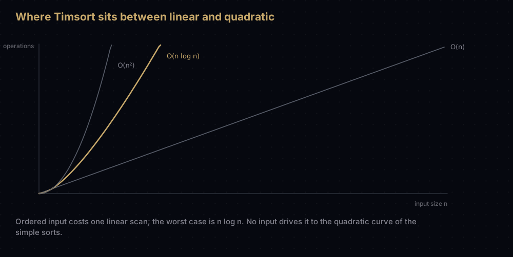
Timsort finds those stretches, calls them runs, and merges them. Sorted input is one run, so it finishes in a single scan of n − 1 comparisons. Shuffled input has runs of two or three, so it costs O(n log n) like any other merge sort. It is stable, it needs O(n) scratch memory, and everything interesting about it is in the details: how short runs get padded, which runs get merged and when, and what it does when one run starts winning every comparison.
The idea
A run is a stretch of the list that is already in order. Timsort works in four steps, repeated until the list is consumed.

- Scan for a run starting at the current position. Take the longest stretch you can.
- If that run is shorter than
minrun— a number between 32 and 64 that Timsort computes from the length of any list of 64 elements or more: extend it tominrunelements using binary insertion sort. - Push the run onto a stack of pending runs.
- Merge runs on the stack whenever their lengths break a balance rule, so the merges stay roughly equal-sized.
When the scan reaches the end, merge whatever is still on the stack until one run is left. That run is the sorted list.
Step 1 is where the adaptivity comes from, and it has a subtlety. Timsort accepts two kinds of run:
- An ascending run is any non-decreasing stretch:
[4, 7, 7, 9]counts. - A descending run must be strictly decreasing:
[12, 9, 7, 4]counts,[12, 9, 9, 4]stops after[12, 9].
A descending run is reversed in place the moment it is found, which costs one pass over it and turns it into an ascending run like every other. The strictness is not fussiness. It is the entire reason Timsort is stable. Suppose the run were allowed to be merely non-increasing and the data were records with equal sort keys, say scores 3, 2, 2. Reversing that stretch puts the second 2 in front of the first, and two records that compare equal have just been swapped. Nothing later in the algorithm can undo it. By stopping the descending run at the first pair that is not strictly decreasing, Timsort never reverses equal elements.
Here is a 16-element list and the natural runs it contains before Timsort touches anything:
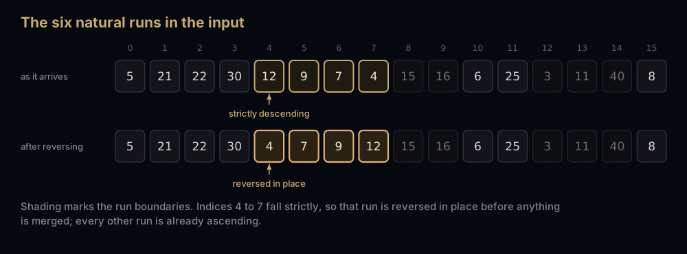
Six runs, one of them descending, one of them a leftover single element. That count (the number of natural runs, usually written ρ) is what decides how much work the sort has to do. One run means one scan. Sixteen runs of one element each means a full merge sort.
Watching it work
Sort [5, 21, 22, 30, 12, 9, 7, 4, 15, 16, 6, 25, 3, 11, 40, 8].
Real Timsort would compute minrun = 16 for a list this short, for any list under 64 elements, minrun is the whole length, so Timsort just binary-insertion-sorts it and stops. To see the merging machinery, force minrun = 4.
Run 1, from index 0. 5, 21, 22, 30 ascends, and 30 > 12 ends it. Length 4, which already meets minrun. Push it. The stack holds runs of [4].
Run 2, from index 4. 12 > 9, so this is a descending run. It extends while it keeps strictly falling: 9 > 7 > 4, and then 4 < 15 stops it. The run [12, 9, 7, 4] is reversed in place to [4, 7, 9, 12]. Push it. The stack holds [4, 4].
The stack now breaks its balance rule (with two runs, the older one must be strictly longer than the newer, and 4 is not longer than 4), so the two are merged into one run of 8: [4, 5, 7, 9, 12, 21, 22, 30]. The stack holds [8].
Run 3, from index 8. 15, 16 ascends and 16 > 6 stops it. Length 2, short of minrun. So the next two elements are absorbed by binary insertion sort: 6 goes to the front, 25 goes to the back, giving [6, 15, 16, 25]. Push it. The stack holds [8, 4], which is balanced — 8 is longer than 4 — so nothing is merged.
Run 4, from index 12. 3, 11, 40 ascends and 40 > 8 stops it. Length 3, one short. Binary insertion sort absorbs 8 into position, giving [3, 8, 11, 40]. Push it. The stack holds [8, 4, 4].
Now the balance rule fires twice. The oldest of the top three runs must be longer than the other two combined, and 8 is not longer than 4 + 4. So the two 4s merge into [3, 6, 8, 11, 15, 16, 25, 40], leaving [8, 8], which breaks the two-run rule as well. Those merge into the finished list.
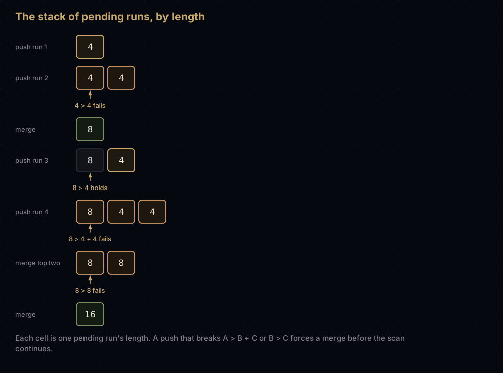
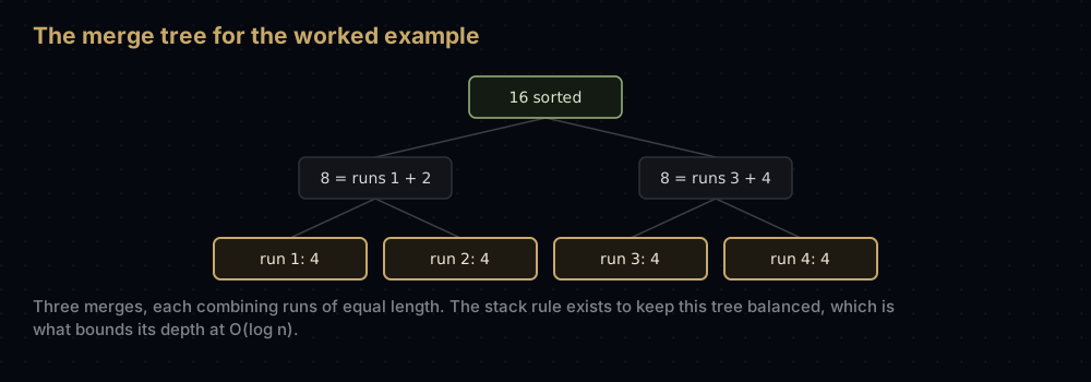
Four runs, three merges, and the merges were 4+4, 4+4 and 8+8: perfectly balanced, which is exactly what the stack rule is for. Nothing merged a run of 12 against a run of 1.
The code
What follows is a faithful but simplified model of Timsort, not a translation of CPython's implementation. The real thing is over a thousand lines of C in Objects/listsort.c, sorts in place rather than returning a copy, and folds galloping into the merge loop. This version keeps the four mechanisms that define the algorithm (run detection, minrun, binary insertion sort, and the merge policy), and stays readable.
Start with minrun. CPython's rule is arithmetic on the bit pattern of n: take its top 6 bits, and add 1 if any of the bits below them were set.
def compute_minrun(n: int) -> int:
    """CPython's rule: the top 6 bits of n, plus 1 if any lower bit is set."""
    has_remainder = 0
    while n >= 64:
        has_remainder |= n & 1
        n >>= 1
    return n + has_remainder


for size in [30, 64, 100, 1000, 1024, 1_000_000]:
    minrun = compute_minrun(size)
    runs = -(-size // minrun)  # ceiling division: how many runs that produces
print(f"n = {size:>9} minrun = {minrun:>3} runs = {runs:>6}")n = 30 minrun = 30 runs = 1
n = 64 minrun = 32 runs = 2
n = 100 minrun = 50 runs = 2
n = 1000 minrun = 63 runs = 16
n = 1024 minrun = 32 runs = 32
n = 1000000 minrun = 62 runs = 16130Look at the run counts: 1, 2, 2, 16, 32 — powers of two — and 16,130, which sits just under 16,384. That is the whole point of the rule. If the number of runs is a power of two, the merges pair up perfectly all the way to the top, like a balanced tree. If it were a power of two plus one, the last merge would be a huge run against a tiny one, which is the worst shape a merge tree can have. Choosing minrun in the range 32 to 64 leaves enough freedom to always land on or just under a power of two.
Run detection comes next, and it is where the ascending and strictly-descending rules live.
def count_run(values: list, start: int) -> int:
    """Length of the natural run at `start`, reversing it if it descends.

    An ascending run is any non-decreasing stretch. A descending run has to be
    *strictly* decreasing: reversing a stretch that contained equal values
    would swap them, and that would destroy stability.
    """
    end = start + 1
    if end == len(values):
        return 1

    if values[end] < values[end - 1]:
        while end + 1 < len(values) and values[end + 1] < values[end]:
            end += 1
        values[start:end + 1] = reversed(values[start:end + 1])
    else:
        while end + 1 < len(values) and not values[end + 1] < values[end]:
            end += 1

    return end - start + 1


sample = [5, 21, 22, 30, 12, 9, 7, 4, 15, 16, 6, 25, 3, 11, 40, 8]
print(count_run(sample, 0), sample[0:4])
print(count_run(sample, 4), sample[4:8])
print(count_run(sample, 8), sample[8:10])
print(count_run([2, 2, 2], 0))4 [5, 21, 22, 30]
4 [4, 7, 9, 12]
2 [15, 16]
3The last line is the stability rule in action: three equal values are one ascending run of length 3, never a descending run, so they are never reversed.
Short runs are padded by binary insertion sort: plain insertion sort with the linear search for the insertion point replaced by a binary search.
def binary_insertion_sort(values: list, low: int, high: int, start: int) -> None:
    """Sort values[low:high] in place, given values[low:start] is sorted already."""
    if start <= low:
        start = low + 1

    for index in range(start, high):
        pivot = values[index]
        left, right = low, index
        # Binary search for the slot just after every value that is <= pivot.
        # Going right on ties is what keeps equal values in their input order.
        while left < right:
            middle = (left + right) // 2
            if pivot < values[middle]:
                right = middle
            else:
                left = middle + 1
        # Shift the block one place right, then drop the pivot into the hole.
        values[left + 1:index + 1] = values[left:index]
        values[left] = pivot


short_run = [15, 16, 6, 25]
binary_insertion_sort(short_run, 0, 4, 2)
print(short_run)[6, 15, 16, 25]The start argument is why this is worth doing: the run detector has already established that values[low:start] is sorted, so binary insertion sort resumes from there instead of starting over.
Now the merging. One function merges two adjacent runs, one merges a pair of stack entries, and one enforces the balance rule.
def merge_runs(values: list, start: int, middle: int, end: int) -> None:
    """Merge the sorted values[start:middle] and values[middle:end] in place."""
    left = values[start:middle]
    left_index, right_index, out = 0, middle, start

    while left_index < len(left) and right_index < end:
        # Take from the right run only when it is strictly smaller, so a tie
        # goes to the left run - the one that came first in the input.
        if values[right_index] < left[left_index]:
            values[out] = values[right_index]
            right_index += 1
        else:
            values[out] = left[left_index]
            left_index += 1
        out += 1

    # Whatever is left in the right run already sits in its final place.
    while left_index < len(left):
        values[out] = left[left_index]
        left_index += 1
        out += 1


def merge_at(values: list, stack: list, i: int) -> None:
    """Merge stack entries i and i + 1, replacing both with the combined run."""
    (start_a, len_a), (start_b, len_b) = stack[i], stack[i + 1]
    merge_runs(values, start_a, start_b, start_b + len_b)
    stack[i] = (start_a, len_a + len_b)
    del stack[i + 1]


def merge_collapse(values: list, stack: list) -> None:
    """Merge until the top of the stack satisfies A > B + C and B > C."""
    while len(stack) > 1:
        i = len(stack) - 2
        if ((i > 0 and stack[i - 1][1] <= stack[i][1] + stack[i + 1][1])
                or (i > 1 and stack[i - 2][1] <= stack[i - 1][1] + stack[i][1])):
            # Merge the middle run into whichever neighbour is smaller.
            if stack[i - 1][1] < stack[i + 1][1]:
                i -= 1
            merge_at(values, stack, i)
        elif stack[i][1] <= stack[i + 1][1]:
            merge_at(values, stack, i)
        else:
            return


def merge_force_collapse(values: list, stack: list) -> None:
    """Merge whatever is still pending once the scan reaches the end."""
    while len(stack) > 1:
        i = len(stack) - 2
        if i > 0 and stack[i - 1][1] < stack[i + 1][1]:
            i -= 1
        merge_at(values, stack, i)
And the driver that ties the four steps together.
def timsort(items: list, minrun: int = 0) -> list:
    """Sort a list with a simplified Timsort and return a new list.

    Scans for natural runs, extends short ones to minrun with binary insertion
    sort, then merges them under the stack invariants. Pass `minrun` to override
    the computed value; a small example otherwise never merges at all.
    """
    values = list(items)
    n = len(values)
    if n < 2:
        return values

    min_run = minrun or compute_minrun(n)
    stack = []  # (start index, length) for every pending run, oldest first
    index = 0

    while index < n:
        run_length = count_run(values, index)
        if run_length < min_run:
            # Too short to be worth merging: grow it to minrun by inserting the
            # elements that follow into the sorted prefix, one at a time.
            forced = min(min_run, n - index)
            binary_insertion_sort(values, index, index + forced, index + run_length)
            run_length = forced

        stack.append((index, run_length))
        index += run_length
        merge_collapse(values, stack)

    merge_force_collapse(values, stack)
    return values


data = [5, 21, 22, 30, 12, 9, 7, 4, 15, 16, 6, 25, 3, 11, 40, 8]
print(timsort(data))
print(timsort([]), timsort([7]), timsort([2, 1]))
print(timsort([4, 4, 4, 1]))
print(timsort(data) == sorted(data))[3, 4, 5, 6, 7, 8, 9, 11, 12, 15, 16, 21, 22, 25, 30, 40]
[] [7] [1, 2]
[1, 4, 4, 4]
TrueHow the code maps to the idea
The merge takes from the right run only on a strict <. Equal values therefore always come from the left run, which is the run that appeared earlier in the input. That is the last of the three places where this algorithm could reorder equal elements, and all three are closed off: count_run never reverses a stretch containing equal values, binary_insertion_sort places a value after everything it ties with, and the merge lets the left run win every tie. Together they are the whole stability argument.
class Player:
    """Compares on score alone, so two players with one score are a real tie."""

    def __init__(self, name: str, score: int) -> None:
        self.name = name
        self.score = score

    def __lt__(self, other: "Player") -> bool:
        return self.score < other.score

    def __repr__(self) -> str:
        return f"{self.name}:{self.score}"


table = [Player("ana", 3), Player("bo", 2), Player("cy", 2), Player("dee", 1)]
print(timsort(table, minrun=2))[dee:1, bo:2, cy:2, ana:3]bo still comes before cy. Had count_run accepted a non-increasing run, all four records would have been one falling run, reversed in a single step, and cy would have come out in front of bo with nothing left to fix it.
The stack rule is two inequalities. Writing A, B and C for the third-from-top, second-from-top and top runs, merge_collapse restores A > B + C and B > C before returning. Both are about keeping merges balanced: if a long run were allowed to sit next to a short one, the eventual merge between them would copy the long run for almost no benefit. When the rule is broken, the middle run is merged into whichever neighbour is smaller. That is the if stack[i - 1][1] < stack[i + 1][1] line.
The second half of that condition, the i > 1 clause, checks four runs deep rather than three. That is not decoration; it is a fix, and the story behind it is in the real-world section below.
merge_force_collapse is not optional. The scan pushes runs and merges only when the balance rule demands it, so when the input runs out there are usually several runs still pending. Forgetting the final collapse gives you a list of sorted blocks rather than a sorted list.
Run the driver again with the printing turned on and every claim from the walkthrough can be checked against what actually happens:
def timsort_traced(items: list, minrun: int) -> list:
    """The same driver loop, printing every run it finds and every merge."""
    values = list(items)
    n = len(values)
    stack = []
    index = 0

    def merge_and_report(i: int) -> None:
        (start_a, len_a), (start_b, len_b) = stack[i], stack[i + 1]
        left = values[start_a:start_a + len_a]
        right = values[start_b:start_b + len_b]
        merge_at(values, stack, i)
        print(f"  merge {left}")
        print(f"      + {right}")
        print(f"     -> {values[start_a:start_a + len_a + len_b]}")

    while index < n:
        before = values[index:]
        run_length = count_run(values, index)
        found = values[index:index + run_length]
        if found == before[:run_length]:
            print(f"run at {index:>2}: {found} ascending")
        else:
            print(f"run at {index:>2}: {before[:run_length]} descending, "
                  f"reversed to {found}")

        if run_length < minrun:
            forced = min(minrun, n - index)
            binary_insertion_sort(values, index, index + forced, index + run_length)
            run_length = forced
            print(f"          too short, extended to "
                  f"{values[index:index + run_length]}")

        stack.append((index, run_length))
        index += run_length

        while len(stack) > 1:
            i = len(stack) - 2
            if ((i > 0 and stack[i - 1][1] <= stack[i][1] + stack[i + 1][1])
                    or (i > 1 and stack[i - 2][1] <= stack[i - 1][1] + stack[i][1])):
                if stack[i - 1][1] < stack[i + 1][1]:
                    i -= 1
                merge_and_report(i)
            elif stack[i][1] <= stack[i + 1][1]:
                merge_and_report(i)
            else:
                break
        print(f"  stack holds runs of {[length for _, length in stack]}")

    while len(stack) > 1:
        i = len(stack) - 2
        if i > 0 and stack[i - 1][1] < stack[i + 1][1]:
            i -= 1
        merge_and_report(i)

    return values


print(timsort_traced(data, minrun=4))run at 0: [5, 21, 22, 30] ascending
stack holds runs of [4]
run at 4: [12, 9, 7, 4] descending, reversed to [4, 7, 9, 12]
merge [5, 21, 22, 30]
+ [4, 7, 9, 12]
-> [4, 5, 7, 9, 12, 21, 22, 30]
stack holds runs of [8]
run at 8: [15, 16] ascending
too short, extended to [6, 15, 16, 25]
stack holds runs of [8, 4]
run at 12: [3, 11, 40] ascending
too short, extended to [3, 8, 11, 40]
merge [6, 15, 16, 25]
+ [3, 8, 11, 40]
-> [3, 6, 8, 11, 15, 16, 25, 40]
merge [4, 5, 7, 9, 12, 21, 22, 30]
+ [3, 6, 8, 11, 15, 16, 25, 40]
-> [3, 4, 5, 6, 7, 8, 9, 11, 12, 15, 16, 21, 22, 25, 30, 40]
stack holds runs of [16]
[3, 4, 5, 6, 7, 8, 9, 11, 12, 15, 16, 21, 22, 25, 30, 40]Galloping mode
The code above leaves out one mechanism, and it is the one that gives Timsort its most dramatic wins. Consider merging a run of 100,000 sorted timestamps with a run of 20 late arrivals. A plain merge walks the big run one element at a time, spending a comparison on each: 100,000 comparisons to move data that was already in the right order.
Timsort watches for this. It counts how many times in a row the same run has won the comparison, and when that count reaches 7 it switches into galloping mode. Instead of comparing one element at a time, it searches ahead exponentially: is the other run's next value bigger than the one 1 place ahead? 2 places? 4, 8, 16, and so on. Once a probe overshoots, the answer is bracketed between the last two probes, and a binary search of that gap finds the exact split point. Then the whole block is copied in one move.
def gallop_right(key: int, run: list) -> tuple:
    """Where `key` belongs in a sorted run, by doubling then binary search.

    Returns (index, comparisons) so the saving over a plain scan is visible.
    """
    comparisons = 0
    offset = 1

    # Probe at offsets 1, 2, 4, 8, ... until the key is overshot.
    while offset <= len(run):
        comparisons += 1
        if key < run[offset - 1]:
            break
        offset *= 2

    # The answer lies between the last two probes. Binary search that gap.
    low, high = offset // 2, min(offset, len(run))
    while low < high:
        middle = (low + high) // 2
        comparisons += 1
        if key < run[middle]:
            high = middle
        else:
            low = middle + 1

    return low, comparisons


long_run = list(range(1000))
for key in [5, 100, 900]:
    where, comparisons = gallop_right(key, long_run)
    print(f"key {key:>3} belongs at index {where:>3}: {comparisons:>2} comparisons "
f"galloping, {where + 1:>3} scanning")key 5 belongs at index 6: 6 comparisons galloping, 7 scanning
key 100 belongs at index 101: 14 comparisons galloping, 102 scanning
key 900 belongs at index 901: 19 comparisons galloping, 902 scanning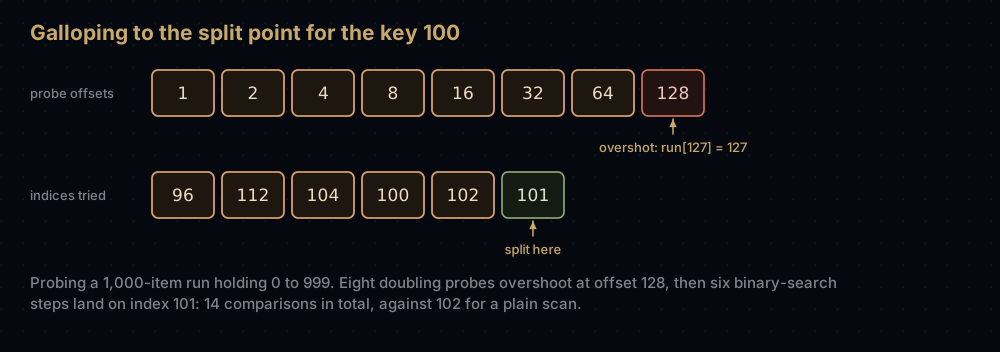
The doubling phase and the binary search each cost about log₂ k comparisons, so finding a block of k elements to copy costs about 2 log₂ k instead of k. The first row of that output is the reason galloping is not always on: for a block of 6 elements it saved a single comparison, and the bookkeeping costs more than that. Hence the threshold of 7 consecutive wins, and hence CPython's adaptive tuning: the threshold goes down while galloping keeps paying and up when it stops, so data that alternates between the two runs never pays for it.
bisect.bisect_right in the standard library does the binary-search half of this, and bisect.insort is a ready-made binary insertion. Neither gallops: bisect halves the whole range every time, at log₂ n comparisons whatever the answer turns out to be, where galloping probes outward from the previous split point so a nearby answer costs only about 2 log₂ of the distance to it.
Complexity
Best case: O(n). An already-sorted list is one ascending run. count_run walks it to the end in n − 1 comparisons, the run is longer than minrun so nothing is inserted, one run goes on the stack, and there is nothing to merge. A reversed list is the same cost plus one linear reversal. No other comparison sort in this series matches that on both inputs.
Worst case: O(n log n). Two facts give the bound. First, the stack rule keeps merges balanced, so the merge tree has depth O(log n) rather than degenerating into a chain. Second, every merge costs at most one comparison and at most one move per element it outputs, so a whole level of the merge tree costs O(n). Multiply and you get O(n log n).
The padding phase does not change that bound, though it is worth counting, because on random data it is where most of the comparisons actually go. Each of the n/minrun blocks is finished by binary insertion sort at O(minrun log minrun) comparisons and O(minrun²) moves, which across all the blocks is O(n log minrun) comparisons and O(n · minrun) moves. minrun never exceeds 64, so both are O(n).
The balance claim is worth checking rather than trusting. The rule says each run must be longer than the two above it on the stack combined, so the shortest possible stack is 1, 2, 4, 7, 12, 20, 33: each entry the sum of the previous two plus one, which is Fibonacci growth. Run lengths that grow like φ ≈ 1.618 to the power of the stack depth mean the stack is never deep:
smallest = [1, 2]
while sum(smallest) < 1_000_000_000:
    # Every run below the top must be longer than the two runs above it combined.
    smallest.append(smallest[-1] + smallest[-2] + 1)
print(f"{len(smallest)} pending runs need at least {sum(smallest):,} elements")41 pending runs need at least 1,134,903,126 elementsSince 41 runs need more than a billion elements, a billion-element list never holds more than 40 pending runs. That is why the stack can be a small fixed-size array, and why no run ever waits long before being merged into something close to its own size.
The sharper statement of the running time is O(n + n log ρ), where ρ is the number of natural runs in the input. Both bounds above are special cases: ρ = 1 gives O(n), and a uniformly shuffled list has natural runs averaging about two and a half elements, so ρ ≈ n/2.4 and n log ρ is O(n log n). ρ is not the number of runs the merge stack sees: on shuffled input of 1,024 elements ρ is around 420, but minrun padding glues those fragments into 32 blocks of 32 before a single merge happens. ρ measures the order the input already had; n/minrun measures how many runs the merge tree is built from. Proving any of this rigorously is harder than it looks. The first complete proof that Timsort is O(n log n) came from Auger, Nicaud and Pivoteau in 2015 (thirteen years after Tim Peters wrote it, by which point it was running on every Python installation on the planet), and the run-sensitive bound took a few more years to settle.
Space: O(n). The merge needs somewhere to put one of the two runs while it overwrites their combined slot. CPython copies whichever run is shorter, so the buffer never exceeds n/2 elements; the version above always copies the left run, which is simpler and has the same O(n) bound. The run stack adds O(log n) on top. This is Timsort's real cost, and it is not avoidable: it is a merge sort.
Counting comparisons across input shapes shows all of this at once. The wrapper class below counts every < performed on an element, so the same measurement works on this implementation and on the built-in sorted().
class Counted:
    """An int wrapper that counts every < performed on it."""

    comparisons = 0

    def __init__(self, value: int) -> None:
        self.value = value

    def __lt__(self, other: "Counted") -> bool:
        Counted.comparisons += 1
        return self.value < other.value


def comparisons_for(sort, values: list) -> int:
    """Run `sort` over wrapped values and report the comparisons it needed."""
    Counted.comparisons = 0
    result = sort([Counted(value) for value in values])
    assert [item.value for item in result] == sorted(values)
    return Counted.comparisons


size = 1024
cases = [
    ("already sorted", list(range(size))),
    ("reversed", list(range(size - 1, -1, -1))),
    ("two runs interleaved", list(range(0, size, 2)) + list(range(1, size, 2))),
    ("sorted, 20 appended", list(range(size - 20)) + [(i * 401) % size for i in range(20)]),
    ("shuffled", [(i * 401) % size for i in range(size)]),
]

print(f"{'input (n = 1024)':<22}{'this timsort':>14}{'sorted()':>10}")
for label, values in cases:
    print(f"{label:<22}{comparisons_for(timsort, values):>14}"
          f"{comparisons_for(sorted, values):>10}")
print(f"{'n log2 n':<22}{size * 10:>14}")input (n = 1024) this timsort sorted()
already sorted 1023 1023
reversed 1023 1023
two runs interleaved 2046 2046
sorted, 20 appended 2069 1325
shuffled 8927 8946
n log2 n 10240Every number there is explainable. Sorted and reversed both cost exactly n − 1 = 1,023: one run, no merges. The interleaved case costs 1,023 to find the two 512-element runs and 1,023 to merge them, because interleaved data forces a comparison for every output slot. The shuffled case splits into 3,856 comparisons building 32 runs of 32 with binary insertion sort and 5,071 merging them across five levels: just under the ceiling of 5 × 1,024.
The fourth row is the one to look at. A sorted list with 20 scattered values appended costs this implementation 2,069 comparisons and CPython 1,325. That gap of 744 is galloping: CPython skips over the long stretches of the big run instead of walking them.
When to use it, and when not to
In Python, use it by calling sorted(items) or items.sort(). That is the entire recommendation. The C implementation will beat this Python one by a factor of a hundred or more, it is better tested than anything you will write, and key= handles almost every ordering you need.
Write it yourself only to learn it, or when you are implementing a sort in a language whose standard library does not offer a stable adaptive one.
Timsort is the wrong algorithm when memory is the constraint. It needs up to n/2 elements of scratch space; heap sort gives you O(n log n) with O(1) extra memory, at the cost of stability and cache locality.
It is the wrong algorithm when the data is genuinely random and stability does not matter. On uniformly shuffled input the run detector finds runs averaging two or three elements and rarely anything longer — in a shuffled list of 1,024 the longest natural run is typically about six — so all that machinery is overhead on top of a plain merge sort, and an in-place quick sort variant — which is what C++ std::sort and Rust's sort_unstable use — will usually be faster because it moves less memory.
It is a poor choice to implement from scratch under time pressure. The full algorithm has many more edge cases than the version above: two merge directions, the adaptive gallop threshold, and a run stack whose invariant is subtle enough to have been wrong in production for years. If you need a hand-written sort in a hurry, merge sort gives you the same guarantees minus the adaptivity, in a fifth of the code.
Where it shows up in the real world
CPython. list.sort() and sorted() are Timsort, in Objects/listsort.c. Every sorted() call in every Python program on earth runs it, including the sorted() calls in this post's own test assertions.
Java, and therefore Android. java.util.Arrays.sort on an array of objects, and Collections.sort, have used a port of Timsort since Java 7. Sorting an array of primitives uses dual-pivot quicksort instead: no stability requirement, no allocation. Android's runtime inherits the same class.
V8, and therefore Chrome and Node.js. JavaScript's Array.prototype.sort moved to Timsort in V8 7.0 (2018), replacing an unstable quicksort that had been used for larger arrays. ECMAScript has required a stable sort since ES2019.
The bug a verifier found
In 2015 a group of researchers (de Gouw, Rot, de Boer, Bubel and Hähnle) tried to prove Java's Timsort correct with the KeY program verifier. The proof would not close, and the reason was real: the loop that restores the stack invariant only examined the top three runs, which is not enough to guarantee the invariant holds further down the stack. Since the run stack is a fixed-size array sized from that invariant, a violated invariant lets more runs pile up than there are slots, and java.util.Arrays.sort throws ArrayIndexOutOfBoundsException. They published an input that triggers it: an array of tens of millions of elements with carefully chosen run lengths. The algorithm had been shipping in Java since 2011 and in Python since 2003.
OpenJDK's response was to enlarge the stack so the overflow could not be reached. The paper's own fix was to check one level deeper, which is the four-run condition in merge_collapse above, and that version was machine-checked. CPython was never reported to crash from it in practice: its run stack is sized for lists far larger than any that fits in memory.
Python then went further. Since Python 3.11, list.sort() uses a powersort merge policy, from a 2018 paper by Munro and Wild. Instead of restoring inequalities between neighbouring runs, powersort computes, from where a run boundary falls in the list, what depth that boundary would have in a near-optimal merge tree, and merges accordingly. Run detection, minrun, binary insertion sort and galloping are all unchanged: only the decision about which runs to merge next is different. The result is provably close to the best possible merge order for the run lengths the data actually has, and it retires the invariant that caused the bug.
Common mistakes
Letting descending runs be non-increasing. Writing the descent check as values[end + 1] <= values[end] gains you slightly longer runs and silently loses stability, because the reversal then swaps equal elements. Sorting a table by one column and then another is where it shows up, long after the change.
Forgetting to reverse a descending run. Detecting it and pushing it as-is puts a backwards block on the stack, and every merge afterwards produces garbage. There is no error, just wrong output.
Extending a run past the end of the list. The pad step must use min(minrun, n - index). Without the min, the last run of a list whose length is not a multiple of minrun reaches past the end.
Merging non-adjacent runs. The merge policy may only combine runs that are neighbours in the list. Merging stack entries 0 and 2 would interleave elements across the run in between, which destroys the ordering rather than building it.
Skipping the final forced merge. The stack usually has several runs left when the scan ends. Skipping the collapse returns a list of sorted blocks that looks nearly right in a spot check.
Trusting the top three runs. As above: the invariant has to be restored down the stack, not just at its top. Nobody caught this one until a formal verifier did, thirteen years after Tim Peters wrote it, so it is not an embarrassing mistake to make, but the fix is one extra condition, so make it.
Practice
- Count the natural runs in a list — the value of ρ — by calling run detection repeatedly, and check that an already-sorted list gives 1.
- Modify
count_runto accept non-increasing descending runs, then find an input of records with equal keys where the result is no longer stable. - Add a
keyparameter totimsortso it sorts bykey(item)the waysorted()does, and confirm it matchessorted(items, key=...)on random data. - Wire
gallop_rightintomerge_runs: count consecutive wins by one run, and when a run wins 7 in a row, gallop to find how many of its elements to copy in one block. Compare comparison counts on a 1,000-element run merged with a 10-element one. - Implement powersort's merge rule instead of
merge_collapse, and compare the total number of elements moved on inputs whose runs have very unequal lengths.
Summary
Timsort is a merge sort that starts from the order the data already has. Find the runs, pad short ones to 32-to-64 elements with binary insertion sort, merge under a rule that keeps the merges balanced, and gallop when one run is winning everything. That buys O(n) on sorted data, O(n log n) at worst, and stability throughout, for O(n) scratch memory and a great deal of complexity, which is exactly why you should call sorted() rather than write it.
| Difficulty | Hard |
| Best case | O(n) — one natural run, found in n − 1 comparisons, zero merges |
| Average case | O(n log n) — about n/minrun runs merged over log(n/minrun) levels |
| Worst case | O(n log n) — the stack rule bounds the merge tree depth at O(log n) |
| Run-aware bound | O(n + n log ρ) for ρ natural runs |
| Space | O(n) — a merge buffer of at most n/2, plus an O(log n) run stack |
| Stable | Yes — strictly descending runs, and ties won by the left run |
| In place | No |
| Adaptive | Yes — this is the whole point of the algorithm |
| Data structure | List / array with O(1) indexing |
| Use it when | You are sorting in Python at all, or need a stable adaptive sort |
| Avoid it when | Memory is tight, or data is random and stability is irrelevant |
| Real-world use | CPython sorted(), Java Arrays.sort for objects, Android, V8 |
| Python equivalent | sorted(items) / items.sort(), in C, with powersort since 3.11 |
Everything in this post is one idea applied four times: do not redo work the input has already done. Runs exploit existing order, minrun keeps the merge tree balanced, the stack rule keeps merge sizes even, and galloping skips comparisons whose answer is already predictable.
Keep reading
- Merge Sort in Python — the merge that Timsort is built on, with the O(n log n) argument from first principles.
- Insertion Sort in Python — the sort that builds every short run, and why it beats everything on tiny inputs.
- Binary Search in Python — the halving search behind binary insertion and the second half of galloping.
- Quick Sort in Python — the faster-on-random-data alternative, and the stability it gives up.
- Big O Notation — the counting arguments used to justify every bound above.


