Insertion sort is the algorithm you already know. If you have ever slid a new playing card into place among the ones already in your hand, you have run it. What you probably do not know is that it is not a toy: CPython's list.sort(), the C++ standard library's std::sort and Java's Arrays.sort all contain an insertion sort, and all three reach it on ordinary inputs.
That is a strange thing to be true of an O(n²) algorithm, and the explanation is the most useful idea here. O(n²) is insertion sort's worst case, not its behaviour. Its real cost is proportional to how far the input is from sorted: a phrase that can be made exact. Already-ordered data finishes in one linear pass. Data where nothing sits more than 16 places from home is linear again. Only genuinely scrambled input costs quadratic time.
So it is worth learning properly: the shifting inner loop, the counting argument behind every bound, the binary-search variant that cuts comparisons without cutting the running time, and why production sorting code falls back to it below a few dozen elements.
The idea
Split the list in two: a sorted prefix on the left, and an untouched remainder on the right. At the start the prefix is just the first item, which is trivially sorted.
Now repeat one step. Take the first item of the remainder — call it the key — and slide it left through the prefix until it is in the right place, moving everything larger than it one slot right to make room. The prefix is now one item longer and still sorted. Do that until the remainder is empty.
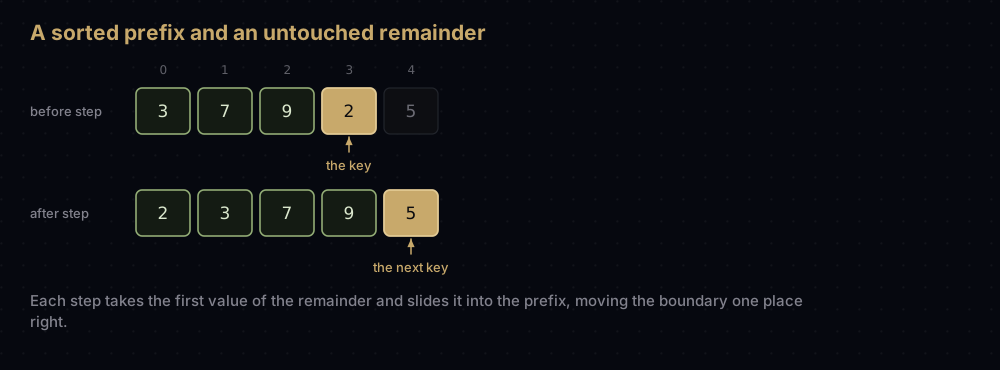
That is the whole algorithm. Here is why it works:
After step i, the first i + 1 items are sorted among themselves. Not in their final positions — a small value still in the remainder will push into them later — but in order relative to each other. When the remainder runs out, the prefix is the whole list.
Two details decide everything about its performance:
- The inner loop stops at the first value not larger than the key. It does not scan the rest of the prefix. On data that is already close to sorted, that stop comes after one comparison and the whole step costs O(1).
- Values are shifted, not swapped. A swap is three memory writes; a shift is one. The key is copied out once at the start of the step and written back once at the end, however far it travels.
Watching it work
Take [7, 3, 9, 2, 5]. The sorted prefix starts as just [7].
Step 1, key = 3. Compare with 7. Larger, so 7 shifts right into index 1 and the gap moves to index 0. Nothing is further left, so 3 goes into the gap: [3, 7, 9, 2, 5]. One comparison, one shift.
Step 2, key = 9. Compare with 7. Not larger, so the loop stops immediately and 9 is written back where it already was. One comparison, zero shifts — the cheap case, and on sorted input every step looks like this.
Step 3, key = 2. Compare with 9, shift. Compare with 7, shift. Compare with 3, shift. The gap has walked all the way to index 0, so 2 is written there: [2, 3, 7, 9, 5]. Three comparisons, three shifts — the expensive case, and on reversed input every step looks like this.
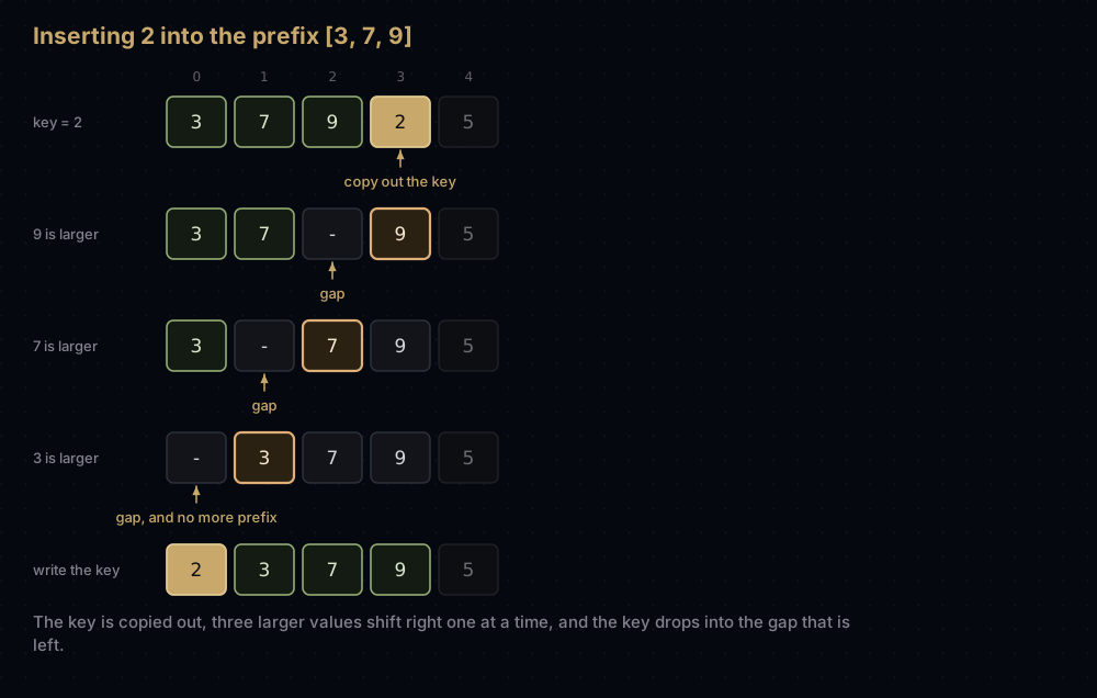
Step 4, key = 5. Compare with 9, shift. Compare with 7, shift. Compare with 3 — not larger, stop. The gap is at index 2, so 5 goes there: [2, 3, 5, 7, 9]. Three comparisons, two shifts.
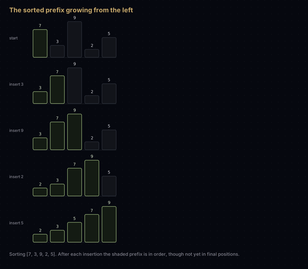
Eight comparisons and six shifts in total. Hold on to that six: the pairs that were in the wrong order in [7, 3, 9, 2, 5] are (7,3), (7,2), (7,5), (3,2), (9,2) and (9,5) — six of them, and that is not a coincidence.
The code
def insertion_sort(items: list[int]) -> list[int]:
    """Sort ascending by inserting each item into an already-sorted prefix.

    Sorts a copy so the caller's list is untouched; drop the copy and return
    None to sort genuinely in place.
    """
    values = list(items)

    for index in range(1, len(values)):
        key = values[index]
        # values[0:index] is already sorted. Walk left through it, shifting
        # every value larger than the key one slot right. The gap left behind
        # when the walk stops is exactly where the key belongs.
        position = index - 1
        while position >= 0 and values[position] > key:
            values[position + 1] = values[position]
            position -= 1
        values[position + 1] = key

    return values


print(insertion_sort([7, 3, 9, 2, 5]))
print(insertion_sort([]))
print(insertion_sort([4]))
print(insertion_sort([2, 2, 1]))[2, 3, 5, 7, 9]
[]
[4]
[1, 2, 2]Here it is again with a print inside, so you can check the walkthrough against what the machine really does:
def insertion_sort_traced(items: list[int]) -> list[int]:
    """Insertion sort that reports the list after every insertion."""
    values = list(items)

    for index in range(1, len(values)):
        key = values[index]
        position = index - 1
        shifts = 0
        while position >= 0 and values[position] > key:
            values[position + 1] = values[position]
            position -= 1
            shifts += 1
        values[position + 1] = key
        print(f"insert {key}: {shifts} shift(s) -> {values}")

    return values


insertion_sort_traced([7, 3, 9, 2, 5])insert 3: 1 shift(s) -> [3, 7, 9, 2, 5]
insert 9: 0 shift(s) -> [3, 7, 9, 2, 5]
insert 2: 3 shift(s) -> [2, 3, 7, 9, 5]
insert 5: 2 shift(s) -> [2, 3, 5, 7, 9]How the code maps to the idea
The outer loop starts at 1, not 0. Index 0 is the initial prefix, and a one-item list is already sorted, so there is nothing to insert on the first step.
key = values[index] must happen before any shifting. This is the line beginners drop. The shifting writes into values[index], so a later read returns whatever got shifted in. Copy it out first and the loop can trample the slot freely.
The while condition has two halves. position >= 0 guards the walk against running off the left end; values[position] > key is the actual test. The guard is the half that must be there: without it the walk reads values[-1], which in Python is the last item of the list rather than an error. Writing it first also lets and short-circuit, so that out-of-range read never happens at all, and in C or Java, where the same read is genuinely out of bounds, putting it first is mandatory rather than tidy.
values[position + 1] = key uses position + 1, not position. When the loop exits, position points at the item that stopped it: the last item not larger than the key, or -1 if the key beat everything. The gap is always one slot to its right.
The comparison is strictly >, not >=. A stored value equal to the key is never shifted past it, so the key comes to rest after its equals. Items that compare equal keep the order they arrived in, which is the definition of a stable sort:
def sort_by_score(rows: list[tuple[str, int]]) -> list[tuple[str, int]]:
    """Insertion sort on the score field only, leaving ties in input order."""
    values = list(rows)

    for index in range(1, len(values)):
        key = values[index]
        position = index - 1
        # Strictly greater: a stored row equal on score is never shifted past
        # the key, so equal scores keep the order they arrived in.
        while position >= 0 and values[position][1] > key[1]:
            values[position + 1] = values[position]
            position -= 1
        values[position + 1] = key

    return values


print(sort_by_score([("ana", 7), ("bo", 3), ("cy", 7), ("di", 3), ("eve", 5)]))[('bo', 3), ('di', 3), ('eve', 5), ('ana', 7), ('cy', 7)]ana was entered before cy and both scored 7; ana still comes first. Change > to >= and the sort is still correct, but the tie order flips. Stability is what lets you sort by one field then another without undoing the first sort.
The edge cases need no code. An empty or one-item list makes range(1, 0) or range(1, 1) empty, so the outer loop never runs and the input comes straight back. Both are in the first output above.
Complexity
Insertion sort has two separate costs, and keeping them apart is what makes the analysis honest.
Shifts. A pair of positions (i, j) with i before j but values[i] > values[j] is called an inversion: a pair in the wrong order. Every shift moves one value one place right, past exactly one value that belongs after it, destroying exactly one inversion. The sort ends when none are left. So the total number of shifts equals the number of inversions in the input, exactly. Six inversions in [7, 3, 9, 2, 5], six shifts.
Comparisons. Each step does one comparison per shift, plus one more for the test that stopped the walk unless the walk ran off the left end, where there is no final test. So comparisons are at least n − 1 and at most shifts + (n − 1).
Everything follows from those two sentences.
Worst case: O(n²). A reversed list has every pair inverted: step i shifts all i values before it, so the total is 1 + 2 + … + (n − 1) = n(n − 1) / 2, which is (n² − n) / 2, which is O(n²).
Average case: O(n²). For a random ordering each of the n(n − 1) / 2 pairs is inverted with probability ½, so the expected number of inversions is n(n − 1) / 4. Half of the worst case is still quadratic.
Best case: O(n). An already-sorted list has zero inversions, so zero shifts, and each step does one comparison and stops: n − 1 comparisons and nothing else. No flag, no special case: the inner loop's stopping condition gives it away for free, which is what makes insertion sort adaptive.
Space: O(1). One key, one position, one loop counter, whatever the input size. The version above returns a copy for convenience, costing O(n); delete the list(items) call and it is genuinely in place.
Here are all three, measured:
def insertion_sort_counted(items: list[int]) -> tuple[int, int]:
    """Count the comparisons and shifts insertion sort needs for `items`."""
    values = list(items)
    comparisons = shifts = 0

    for index in range(1, len(values)):
        key = values[index]
        position = index - 1
        while position >= 0:
            comparisons += 1
            if values[position] <= key:
                break
            values[position + 1] = values[position]
            position -= 1
            shifts += 1
        values[position + 1] = key

    return comparisons, shifts


def reversed_blocks(size: int, block: int) -> list[int]:
    """The values 1..size with each run of `block` consecutive values flipped.

    Nothing ends up more than block - 1 places from where it belongs, which
    makes this a controlled way to build nearly-sorted input.
    """
    values = list(range(1, size + 1))
    for start in range(0, size, block):
        values[start:start + block] = reversed(values[start:start + block])
    return values


shuffled = [9, 2, 14, 5, 1, 16, 7, 11, 3, 13, 6, 15, 4, 12, 8, 10]

print(f"{'input (16 items)':<22}{'comparisons':>12}{'shifts':>8}")
for label, data in [
    ("already sorted", list(range(1, 17))),
    ("blocks of 4 reversed", reversed_blocks(16, 4)),
    ("shuffled", shuffled),
    ("fully reversed", list(range(16, 0, -1))),
]:
    comparisons, shifts = insertion_sort_counted(data)
print(f"{label:<22}{comparisons:>12}{shifts:>8}")input (16 items) comparisons shifts
already sorted 15 0
blocks of 4 reversed 36 24
shuffled 66 53
fully reversed 120 120Sorted input costs 15 comparisons, which is n − 1. Reversed input costs 120, which is 16 × 15 / 2. The shuffled list lands at 53 shifts against an expected 60. The bounds are not approximations here; they are arithmetic.
Nearly sorted input: O(n·k)
Now the result that makes insertion sort useful, not just instructive.
Suppose no value is more than k places from where it belongs. Take any inversion: a value at index i that belongs at p, and a value at a later index j that belongs at an earlier q. Since i is at most k below p, j at most k above q, and q below p, the gap j - i is smaller than 2k. So a value can only be inverted with values within 2k positions of it: fewer than 2kn inversions in the whole list.
Shifts equal inversions, so the sort does fewer than 2kn shifts and 2kn + n comparisons: O(n·k), linear in n for any fixed k. The reversed_blocks helper builds exactly that input, so the claim can be checked:
print(f"{'k':>5}{'shifts':>10}{'n*k/2':>10}")
for k in (1, 3, 7, 15, 1023):
    _, shifts = insertion_sort_counted(reversed_blocks(1024, k + 1))
print(f"{k:>5}{shifts:>10}{1024 * k // 2:>10}") k shifts n*k/2
1 512 512
3 1536 1536
7 3584 3584
15 7680 7680
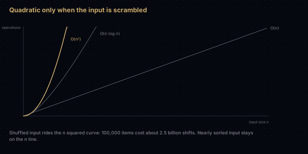
1023 523776 523776Doubling k doubles the work; so does doubling n. It only turns quadratic when k grows with n, which is what the last row shows: k = n − 1, back to n(n − 1) / 2. For 100,000 items:
| Input shape | Shifts, roughly |
|---|---|
| already sorted | 0 |
| nothing more than 16 places from home | under 3.2 million |
| shuffled | 2.5 billion |
| reversed | 5 billion |
Binary insertion sort
The prefix is sorted, so finding the key's slot does not need a linear scan: a binary search can do it in about log₂(i) comparisons instead of up to i. Python's bisect module has this built in.
from bisect import bisect_right, insort


def binary_insertion_sort(items: list[int]) -> list[int]:
    """Insertion sort that locates each slot by binary search.

    Comparisons drop to O(n log n). The shifting is untouched, so the running
    time is still O(n^2).
    """
    values = list(items)

    for index in range(1, len(values)):
        key = values[index]
        # bisect_right lands after any equal values already placed, which is
        # what keeps this variant stable.
        slot = bisect_right(values, key, 0, index)
        # One slice assignment, but it still copies index - slot values.
        values[slot + 1:index + 1] = values[slot:index]
        values[slot] = key

    return values


def binary_insertion_counted(items: list[int]) -> tuple[int, int]:
    """Count comparisons and shifts for the binary-search variant."""
    values = list(items)
    comparisons = shifts = 0

    for index in range(1, len(values)):
        key = values[index]
        low, high = 0, index
        while low < high:
            comparisons += 1
            middle = (low + high) // 2
            if values[middle] <= key:
                low = middle + 1
            else:
                high = middle
        shifts += index - low
        values[low + 1:index + 1] = values[low:index]
        values[low] = key

    return comparisons, shifts


print(binary_insertion_sort([7, 3, 9, 2, 5]))

reverse_16 = list(range(16, 0, -1))
linear_comparisons, linear_shifts = insertion_sort_counted(reverse_16)
binary_comparisons, binary_shifts = binary_insertion_counted(reverse_16)
print(f"linear scan:   {linear_comparisons:>3} comparisons, {linear_shifts:>3} shifts")
print(f"binary search: {binary_comparisons:>3} comparisons, {binary_shifts:>3} shifts")[2, 3, 5, 7, 9]
linear scan: 120 comparisons, 120 shifts
binary search: 49 comparisons, 120 shifts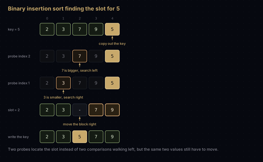
Comparisons fall from 120 to 49: summing log₂(i) over the n steps gives O(n log n) comparisons in every case, worst included. The shifts do not change at all. Still 120, because the values between the slot and the key must physically move however cleverly you located the slot. Total work stays O(n²), so this variant only wins when a comparison is expensive relative to a move: long strings, or records compared through a Python callback. It also gives up the O(n) best case, since a binary search on sorted input still costs log₂(i) comparisons per step rather than one.
That trade-off is not academic: CPython's Timsort uses binary insertion sort precisely because comparing two arbitrary Python objects is expensive.
When to use it, and when not to
Use it when n is small. Below roughly 20 to 50 items it beats merge sort and quick sort in wall-clock time despite the worse growth rate: it allocates nothing, never recurses, walks memory in a straight line, and its whole inner loop is one compare and one move.
Use it when the data is nearly sorted. The O(n·k) result above is the whole argument. Log lines arriving slightly out of order, a leaderboard after a few scores change, objects sorted by depth in a scene where things moved since the last frame: all k-sorted for small k.
Use it when items arrive one at a time. Insertion sort is naturally online: it does not need the whole input before starting. Keeping a list sorted as data streams in is one insertion per arrival, and the standard library does it for you:
leaderboard: list[int] = []
for score in [7, 3, 9, 2, 5]:
    insort(leaderboard, score)
print(leaderboard)[7]
[3, 7]
[3, 7, 9]
[2, 3, 7, 9]
[2, 3, 5, 7, 9]Do not use it on large unsorted data. Sorting 100,000 shuffled items means about 2.5 billion shifts. In production Python the answer is sorted(items) or items.sort(), which run Timsort in C: O(n log n) worst case, stable, adaptive to existing runs. To implement a general-purpose sort yourself, merge sort gives a guaranteed O(n log n) and quick sort the fastest average case.
Against the other two simple sorts: it beats bubble sort on every axis, so there is never a reason to prefer bubble sort. Selection sort is a real choice: it does exactly n − 1 swaps, so it wins when writing is far more expensive than reading, such as sorting records held in flash memory. Everywhere else insertion sort wins, because selection sort's n²/2 comparisons happen however sorted the input already is.
Where it shows up in the real world
CPython's list.sort() and sorted(). Timsort scans for naturally ordered runs. A run shorter than minrun — a value between 32 and 64 derived from the list length — is extended to minrun elements by binary insertion sort before merging. On shuffled data natural runs are only two or three items long, so almost every run is built by insertion sort before any merging happens.
The C++ standard library's std::sort. The libstdc++ implementation is an introsort: quicksort partitioning, a heapsort escape hatch if the recursion gets too deep, and a threshold of 16. Once a partition holds 16 or fewer elements the recursion stops and leaves it unsorted. At the end, one insertion sort runs over the entire array, which by then is 16-sorted, so the O(n·k) result makes that final pass linear.
Java's Arrays.sort. Sorting objects uses TimSort with a binarySort routine: binary insertion sort by another name. Sorting primitives uses a dual-pivot quicksort that switches to insertion sort for small ranges.
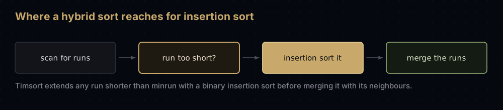
The pattern is the same everywhere: divide and conquer handles the large scale, and insertion sort handles the last few dozen elements, where the better growth rate saves less than the recursion costs.
Common mistakes
Reading values[index] after shifting has started. The key must be copied into a variable first. Skip that and the shift overwrites the value you were placing, so the sort duplicates entries instead of moving them.
Writing the key to values[position]. After the loop, position is the item that stopped the walk, or -1. The gap is at position + 1; writing to position overwrites a value that belongs where it is.
Leaving out the bounds test. while values[position] > key walks straight off the left end, and Python does not stop it (values[-1] is the last item of the list, not an error), so the loop reads the unsorted remainder and either returns a wrong list or raises IndexError a few slots later. The fix is the position >= 0 half of the condition. Writing it second instead of first still sorts correctly in Python, since and demands both halves, but the same line in C or Java reads out of bounds.
Using >= instead of >. Still sorts, but shifts past every equal value, which destroys stability and buys nothing.
Swapping instead of shifting. A chain of swaps sorts correctly, but each step costs three writes instead of one: same complexity class, roughly three times the memory traffic.
Using bisect_left in the binary variant. It lands before equal values, so equal keys end up reversed. bisect_right is what keeps the sort stable.
Practice
- Rewrite
insertion_sortto sort in place, returningNone, and confirm the caller's list is changed. - Add a
descending: bool = Falseparameter that reverses the order, changing only the comparison in thewhilecondition. - Write a function that counts the inversions in a list by running the shift counter, and use it to check that
[3, 1, 2]has 2. - Sort a list of
(surname, first_name)pairs by surname only, then show that two people sharing a surname keep their input order. - Implement Shell sort: insertion-sort elements spaced
gapapart, for gaps of 4, then 2, then 1. Compare its shift count with plain insertion sort on a reversed list of 64 items, and explain the difference using the O(n·k) result.
Summary
Insertion sort is the simple sort that survived. Its cost is the number of inversions in the input, which makes it linear on ordered data, O(n·k) on nearly-ordered data, and quadratic only on genuinely scrambled input. That profile is exactly what a hybrid sort needs for its base case, which is why Python, C++ and Java all ship one inside their standard sort.
| Difficulty | Easy |
| Best case | O(n) — sorted input, n − 1 comparisons and zero shifts |
| Average case | O(n²) — about n(n − 1) / 4 inversions to undo |
| Worst case | O(n²) — reversed input, n(n − 1) / 2 shifts |
| Nearly sorted | O(n·k) — nothing further than k from home |
| Space | O(1) — one key and one index, shifts in place |
| Stable | Yes — strict > never moves an equal value past the key |
| In place | Yes |
| Adaptive | Yes, with no extra code — the inner loop just stops early |
| Online | Yes — items can be inserted as they arrive |
| Data structure | List / array with O(1) indexing |
| Use it when | n is under ~50, the data is nearly sorted, or it arrives one item at a time |
| Avoid it when | n is large and the order is arbitrary |
| Real-world use | The small-run base case inside CPython's Timsort, libstdc++ std::sort and Java's Arrays.sort |
| Python equivalent | sorted(items) / items.sort(), or bisect.insort for one-at-a-time inserts |
Learn the inversion argument here and you get three later results for free: why Timsort hunts for existing runs, why quick sort can afford to leave small partitions unsorted, and why "already sorted" is a case worth testing in every sort you write.
Keep reading
- Bubble Sort in Python — the other adjacent-comparison sort, and why insertion sort replaces it everywhere.
- Selection Sort in Python — the simple sort with the fewest writes, and the one real alternative here.
- Binary Search in Python — the halving search behind the binary insertion variant, from first principles.
- Merge Sort in Python — how restructuring the problem buys a guaranteed O(n log n).
- Timsort — what
sorted()really does, including where it insertion-sorts.


