Bubble sort is the first sorting algorithm almost everyone is taught, and the first one almost everyone is told never to use. Both of those are fair. It is genuinely the easiest sort to understand — you can explain it completely in one sentence — and it is genuinely too slow for real work on anything bigger than a few hundred items.
That combination is exactly why it is worth an hour of your time. Bubble sort is the cheapest possible place to learn the three ideas that every later algorithm in this series depends on: that an algorithm has a cost you can count, that the cost grows with the size of the input, and that a small change to a loop can change that growth entirely.
So this post does not just show you the code. It counts the comparisons, explains where the n² comes from, shows the one optimisation that makes the best case linear, and then tells you honestly what to use instead.
The idea
Walk through the list from left to right. At each step, look at the current item and the one next to it. If they are in the wrong order, swap them. When you reach the end, start again from the left.
That is the whole algorithm.
The name comes from what this looks like when you watch it: on every pass, the largest value still out of place gets carried along by the swaps until it hits the end, like a bubble rising to the surface. After the first pass, the largest item in the whole list is definitely in its final position. After the second pass, the two largest are. After n passes, everything is.
Two things follow from this, and they are worth pausing on because they explain the entire performance profile of the algorithm:
- Each pass is guaranteed to place at least one item correctly. That is why the algorithm always terminates.
- A pass can carry a value a long way right, but only one step left. The scan travels rightwards, so a large value rides along with the swaps and can cross the whole list in a single pass. A small value moves left by exactly one position per pass, so one that starts at the far right needs n − 1 passes to reach the front. That asymmetry is why the algorithm is slow.
Watching it work
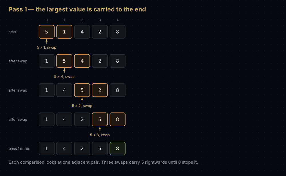
Take the list [5, 1, 4, 2, 8]. The comparisons below are every comparison the algorithm makes, in order.
Pass 1 — compare each adjacent pair across the whole list:
5and1— out of order, swap. The list is now[1, 5, 4, 2, 8].5and4— out of order, swap.[1, 4, 5, 2, 8].5and2— out of order, swap.[1, 4, 2, 5, 8].5and8— already in order, leave it.
Notice that 5 was carried along by three consecutive swaps. That is the bubble. And 8, the largest value, is now at the end where it belongs. It is finished, permanently.
Pass 2 — the last position is already correct, so there is no point comparing it again:
1and4— fine.4and2— swap.[1, 2, 4, 5, 8].4and5— fine.
Pass 3 — the list happens to be fully sorted now, but the algorithm does not know that yet. It compares 1 with 2, then 2 with 4, makes no swaps at all, and that is how it finds out.
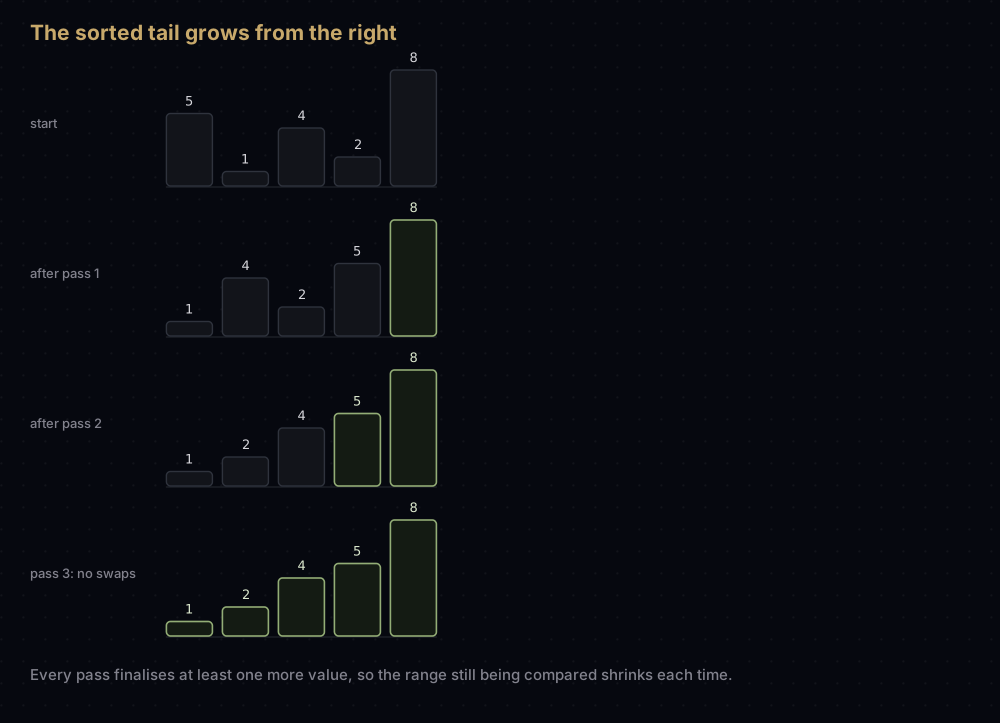
Three passes, nine comparisons, four swaps. The shrinking comparison range matters: pass 1 does 4 comparisons, pass 2 does 3, pass 3 does 2. Nobody re-checks the tail that is already known to be sorted.
The code
Here is the plain version first: the passes and the shrinking range from the walkthrough, but no early exit. On [5, 1, 4, 2, 8] that costs all four passes and 10 comparisons rather than the three passes and nine above, because nothing tells it to stop.
def bubble_sort(items: list[int]) -> list[int]:
    """Sort a list in ascending order by repeatedly swapping adjacent pairs.

    Sorts a copy rather than the caller's list, which is the friendlier
    default; drop the copy and return nothing to sort in place.
    """
    values = list(items)
    n = len(values)

    for pass_number in range(n - 1):
        # Everything from index n - 1 - pass_number onwards is already in its
        # final position, so each pass compares a shorter prefix than the last.
        for index in range(n - 1 - pass_number):
            if values[index] > values[index + 1]:
                values[index], values[index + 1] = values[index + 1], values[index]

    return values


print(bubble_sort([5, 1, 4, 2, 8]))
print(bubble_sort([]))
print(bubble_sort([3]))[1, 2, 4, 5, 8]
[]
[3]This works, and it is always O(n²): even on a list that arrives already sorted, it grinds through every pass.
The fix is one boolean. If a pass completes without swapping anything, then no adjacent pair is out of order, which means the list is sorted, which means you can stop immediately.
def bubble_sort_optimised(items: list[int]) -> list[int]:
    """Bubble sort that stops as soon as a full pass makes no swaps."""
    values = list(items)
    n = len(values)

    for pass_number in range(n - 1):
        swapped = False

        for index in range(n - 1 - pass_number):
            if values[index] > values[index + 1]:
                values[index], values[index + 1] = values[index + 1], values[index]
                swapped = True

        # A clean pass means every adjacent pair is already ordered, and that
        # is the definition of a sorted list. Nothing later can change it.
        if not swapped:
            break

    return values


print(bubble_sort_optimised([5, 1, 4, 2, 8]))
print(bubble_sort_optimised([1, 2, 3, 4, 5]))[1, 2, 4, 5, 8]
[1, 2, 3, 4, 5]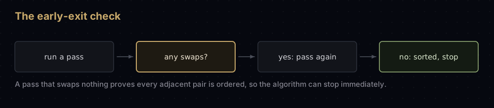
That single flag is the difference between an algorithm that is always O(n²) and one that recognises sorted input in a single linear pass. It costs one variable.
How the code maps to the idea
The outer loop runs the passes. It stops at n - 1 rather than n because after n − 1 items have been placed, the last one has nowhere else to be: a one-item list is sorted by definition.
The inner loop bound, n - 1 - pass_number, is the shrinking range from the walkthrough. Without the - pass_number the code still sorts correctly, it just wastes time re-comparing a tail it has already finished. That subtraction halves the total comparison count.
The swap uses Python's tuple assignment, a, b = b, a. The right-hand side is evaluated completely before anything is assigned, so no temporary variable is needed and there is no order-of-assignment bug to get wrong.
The comparison is strictly >, not >=. This matters more than it looks. With >, two equal values are never swapped, so items that compare equal keep their original relative order, the algorithm is stable. Change it to >= and it still sorts, but it shuffles equal elements needlessly and stability is gone. Stability is what lets you sort a list of records by one field and then another without destroying the first ordering.
Edge cases need no special handling. An empty list makes range(-1) empty, so the loops never run. A one-item list makes range(0) empty, likewise. Both fall out of the arithmetic for free, which is worth checking whenever you write a loop bound.
Let us actually count the work rather than take the complexity claim on faith:
def bubble_sort_counted(items: list[int]) -> tuple[list[int], int, int]:
    """Same algorithm, but also reports comparisons and swaps made."""
    values = list(items)
    n = len(values)
    comparisons = swaps = 0

    for pass_number in range(n - 1):
        swapped = False
        for index in range(n - 1 - pass_number):
            comparisons += 1
            if values[index] > values[index + 1]:
                values[index], values[index + 1] = values[index + 1], values[index]
                swaps += 1
                swapped = True
        if not swapped:
            break

    return values, comparisons, swaps


for label, data in [
    ("random   ", [5, 1, 4, 2, 8]),
    ("sorted   ", [1, 2, 3, 4, 5]),
    ("reversed ", [5, 4, 3, 2, 1]),
]:
    _, comparisons, swaps = bubble_sort_counted(data)
print(f"{label} {comparisons} comparisons, {swaps} swaps")random 9 comparisons, 4 swaps
sorted 4 comparisons, 0 swaps
reversed 10 comparisons, 10 swapsThose three lines are the whole complexity analysis, measured. Sorted input costs one pass. Reversed input costs every pass and swaps on every single comparison.
Complexity
Worst case: O(n²). The worst input is a reversed list, where every comparison results in a swap. Pass 1 makes n − 1 comparisons, pass 2 makes n − 2, and so on down to 1. The total is the sum 1 + 2 + … + (n − 1), which equals n(n − 1) / 2. Multiply that out and you get (n² − n) / 2. Big O throws away the constant ½ and the smaller −n term, leaving O(n²).
You can see this in the numbers above: five reversed items cost 10 comparisons, and 5 × 4 / 2 = 10 exactly.
Average case: O(n²). On randomly ordered input roughly half the pairs are out of order, so you save a constant fraction of the swaps but perform the same n(n − 1) / 2 comparisons. Halving a quantity does not change its growth rate.
Best case: O(n). With the early-exit flag, already-sorted input costs exactly one pass of n − 1 comparisons and zero swaps. Without the flag, the best case is also O(n²). This is entirely a property of that one boolean.
Space: O(1). The algorithm needs a fixed number of variables regardless of input size, and swaps happen inside the list. The version above returns a copy for convenience, which costs O(n); delete the list(items) call and it sorts genuinely in place.
The practical meaning of O(n²) is worth stating in numbers, because "quadratic" is abstract and "a hundred million" is not:
| Items | Comparisons, worst case |
|---|---|
| 10 | 45 |
| 100 | 4,950 |
| 1,000 | 499,500 |
| 10,000 | 49,995,000 |
| 100,000 | 4,999,950,000 |
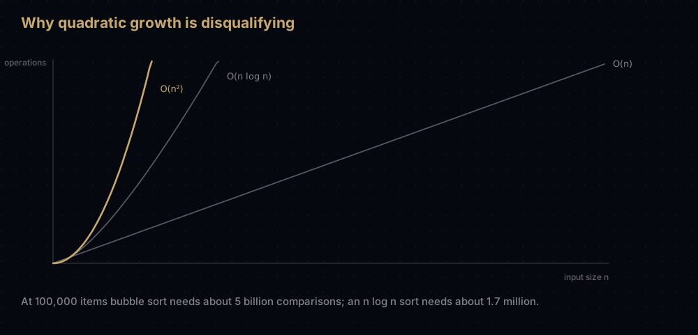
Ten times the data costs a hundred times the work. Merge sort's n log n on those same 100,000 items is about 1.7 million comparisons, roughly three thousand times fewer.
When to use it, and when not to
Use it when you are teaching or learning, when you need a sort you can write correctly from memory with no reference, or when n is genuinely tiny, under about 20 items the difference between any two sorting algorithms is lost in the noise, and simple code has real value.
There is one narrow case where the early-exit version is legitimately good: detecting that a list is already sorted, or nearly so. It confirms a sorted list in a single O(n) pass, and a list with only a handful of adjacent items out of place is fixed in one or two passes.
Do not use it for anything else. In production Python, sorting is sorted(items) or items.sort(), which run Timsort: a hybrid algorithm implemented in C that is O(n log n) worst case, adaptive to already-ordered runs, and stable. It will beat any Python-level sort you write by two or three orders of magnitude, and it is one function call.
If you want a simple hand-written sort that is actually fast on small or nearly-sorted input, insertion sort is the one to reach for. It is barely more code than bubble sort and comfortably faster in practice, which is why real sorting implementations fall back to it for small chunks and bubble sort appears in none of them.
Where it shows up in the real world
Honestly: it does not. No mainstream standard library, database or language runtime sorts with bubble sort, and that is not an oversight.
The nearest thing to a real appearance is in computer graphics and physics engines, where a list of objects sorted by depth or position stays almost sorted from one frame to the next because things move a little. A single bubble pass per frame fixes the few pairs that swapped order, which is O(n) work for a list that is continuously nearly sorted. Even there, insertion sort is the more common choice for exactly the same reason.
Its real role is educational, and it earns that role. Bubble sort is how most people first meet the idea that two programs producing identical output can differ by a factor of a thousand in cost.
Common mistakes
Forgetting the shrinking range. Writing the inner loop as range(n - 1) instead of range(n - 1 - pass_number) still sorts, but it re-compares the sorted tail on every pass and roughly doubles the comparisons.
Going out of bounds. The inner loop reads values[index + 1], so it must stop one short of the end. range(n) instead of range(n - 1) gives you an IndexError on the final iteration.
Setting the swapped flag in the wrong place. It must be reset to False at the start of each pass, inside the outer loop. Initialising it once before the outer loop means it stays True forever after the first swap and the early exit never fires.
Using >= instead of >. Sorts correctly, destroys stability, and performs pointless swaps on equal values.
Comparing non-adjacent items. Swapping values[index] with values[index + 2] does not sort at all: it never compares neighbours, so it happily leaves [1, 0] as [1, 0]. Swapping with the smallest value in the rest of the list is not a bug, but it is not this algorithm either: that is selection sort. Bubble sort's correctness argument depends on only ever swapping neighbours.
Practice
- Rewrite
bubble_sortto sort in place (no copy, returningNone), and confirm the caller's list is modified. - Add a
reverse: bool = Falseparameter that sorts in descending order when set, changing only the comparison. - Write a version that sorts a list of
(name, score)tuples by score, and use its stability to show that names with equal scores keep their input order. - Implement cocktail shaker sort: alternate a left-to-right pass with a right-to-left pass. Measure the comparison count against plain bubble sort on
[5, 4, 3, 2, 1]. - Track the index of the last swap in each pass and use it as the next pass's upper bound. Count how many comparisons this saves on a nearly-sorted list of 50 items.
Summary
Bubble sort is a correct, stable, in-place sort with an unusable growth rate. Learn it for the counting argument (n(n − 1) / 2 comparisons, therefore O(n²)), and for the lesson that one boolean turned its best case from quadratic to linear. Then use sorted() and move on to merge sort or quick sort, where O(n log n) comes from actually restructuring the problem rather than patching the loop.
| Difficulty | Easy |
| Best case | O(n) — one clean pass, only with the early-exit flag |
| Average case | O(n²) — about n(n − 1) / 4 swaps |
| Worst case | O(n²) — reversed input, n(n − 1) / 2 comparisons |
| Space | O(1) — a fixed number of variables, swaps in place |
| Stable | Yes — strict > never reorders equal values |
| In place | Yes |
| Adaptive | Yes, with the early-exit flag |
| Data structure | List / array with O(1) indexing |
| Use it when | Teaching, n under ~20, or checking whether data is already sorted |
| Avoid it when | n is above a few hundred, or performance matters at all |
| Real-world use | Effectively none; occasionally a single pass over nearly-sorted frame data |
| Python equivalent | sorted(items) / items.sort() — Timsort, O(n log n), written in C |
Keep reading
- Insertion Sort in Python — the simple sort that is actually worth using, and the one real algorithms fall back to.
- Selection Sort in Python — the other O(n²) classic, and the one to pick when writes are expensive.
- Merge Sort in Python — where O(n log n) comes from, explained from first principles.
- Big O Notation — the full treatment of the counting argument used above.
- Timsort — what
sorted()actually does, and why it beats everything here.


