Quick sort has the worst headline number of any sorting algorithm people actually use: O(n²) in the worst case, the same bound as bubble sort. It is also the fastest comparison sort in practice, and the algorithm underneath C++'s std::sort, Java's Arrays.sort for primitive arrays, and Go's slices.Sort. Both statements are true, and reconciling them is what this post is for.
The reconciliation is that quick sort's cost is decided by one choice, made over and over: which element to compare everything else against. Choose well and the problem halves at every level, which gives O(n log n). Choose the smallest or largest value every single time and each round strips off one item, which gives O(n²). The algorithm never changes. Only the pivot does.
That one decision is worth 2,698 comparisons against 79,800 on the same 400 items. Both numbers are measured below, by code you can run.
The idea
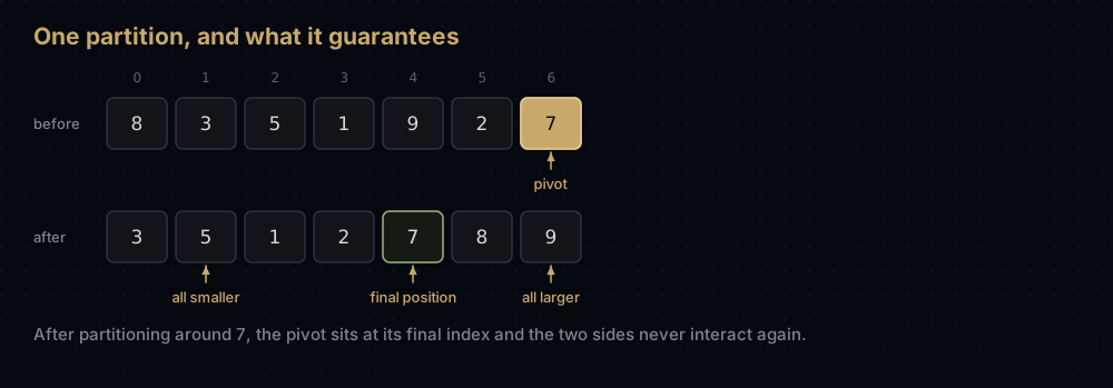
Pick any element of the list and call it the pivot. Rearrange the list so everything smaller than or equal to the pivot sits to its left and everything larger sits to its right. That rearrangement is called partitioning.
Two things are true the moment partitioning finishes, and the whole algorithm rests on them:
- The pivot is in its final position. If four values ended up to its left, it is the fifth item of the sorted list — that is what its rank is. Nothing done later can move it.
- The two sides never interact again. Every value on the left belongs somewhere on the left, and the same holds on the right. So you can sort them independently, with no merging step at the end.
Now do the same to each side, and to their sides, until every part is one element long, and a one-element list is already sorted. That is quick sort in full.
Merge sort is the mirror image: it splits blindly down the middle and does all its real work coming back up, in the merge. Quick sort does all of its work going down, in the partition, and none coming back. That is why quick sort needs no scratch array.
Watching it work
Take [8, 3, 5, 1, 9, 2, 7] and use the last element, 7, as the pivot.
Partitioning keeps one marker: the boundary of the run of values already known to be at most the pivot. That run starts empty. Look at each element in turn, and whenever one belongs in the run, grow the run by a slot and swap the value into it.
8— larger than 7, leave it.[8, 3, 5, 1, 9, 2, 7]3— smaller: the run grows to index 0, so3swaps with8.[3, 8, 5, 1, 9, 2, 7]5— smaller: the run grows to index 1.[3, 5, 8, 1, 9, 2, 7]1— smaller: the run grows to index 2.[3, 5, 1, 8, 9, 2, 7]9— larger, leave it.8and9now sit together, waiting to be jumped over.2— smaller: the run grows to index 3, and2swaps with8.[3, 5, 1, 2, 9, 8, 7]
The run ends at index 3, so the pivot belongs at index 4. Swap it with whatever is in the way: [3, 5, 1, 2, 7, 8, 9].
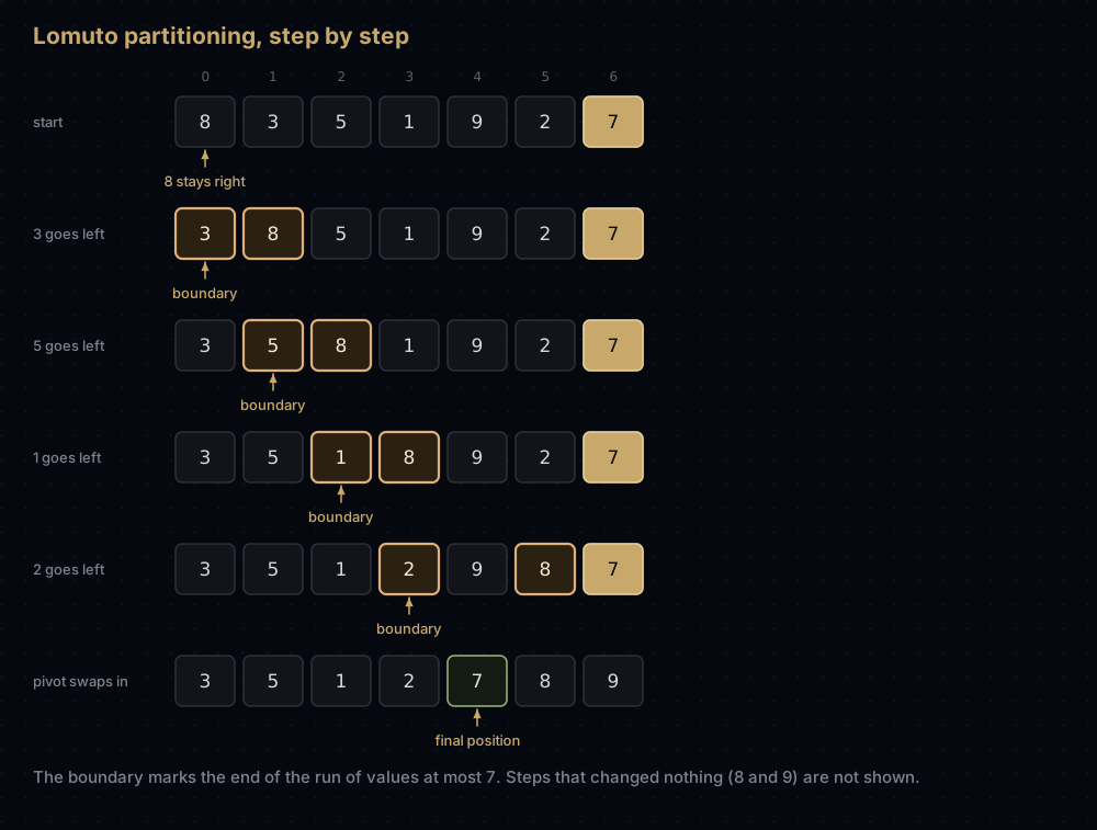
Six comparisons, five swaps, and 7 is finished for good. Now recurse on [3, 5, 1, 2] and [8, 9]. In [3, 5, 1, 2] with pivot 2, only 1 is smaller, so it swaps to index 0 and the pivot follows to index 1: [1, 2, 3, 5]. That leaves [1], done, and [3, 5], which with pivot 5 moves nothing, and neither does [8, 9] with pivot 9.
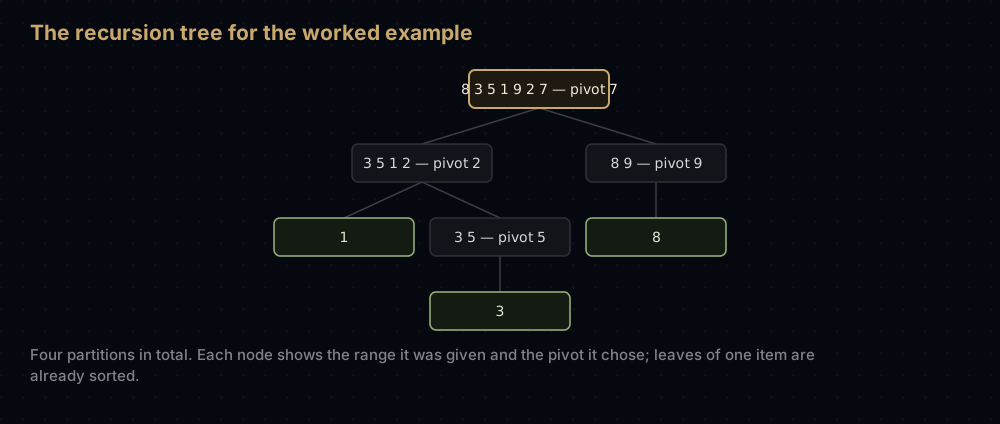
Four partitions, a tree four levels deep, seven items sorted, and nothing ever copied into a second array.
The code
The clearest version is not the real one, so start with it and then fix what is wrong with it.
def quick_sort_simple(items: list[int]) -> list[int]:
    """Sort by picking a pivot, splitting into smaller and larger, and recursing.

    Clear, but wasteful: it builds two fresh lists at every level instead of
    rearranging the one you were given.
    """
    if len(items) <= 1:
        return list(items)

    pivot = items[-1]
    rest = items[:-1]
    smaller = [value for value in rest if value <= pivot]
    larger = [value for value in rest if value > pivot]
    return quick_sort_simple(smaller) + [pivot] + quick_sort_simple(larger)


print(quick_sort_simple([8, 3, 5, 1, 9, 2, 7]))
print(quick_sort_simple([]))
print(quick_sort_simple([4, 4, 4]))[1, 2, 3, 5, 7, 8, 9]
[]
[4, 4, 4]It sorts, and it throws away quick sort's main advantage. Two new lists per level means O(n) extra memory and none of the cache behaviour that makes the real thing fast.
Lomuto partitioning
The real version rearranges the list in place. This is the Lomuto scheme, the one traced above: pivot at the end, one scanning index, one boundary index.
def partition(values: list[int], low: int, high: int) -> int:
    """Lomuto partition of values[low:high + 1] around the pivot values[high].

    Returns the index the pivot ends up at. Everything to its left is <= the
    pivot; everything to its right is greater.
    """
    pivot = values[high]
    boundary = low - 1  # last index of the "<= pivot" run built so far

    for scan in range(low, high):
        if values[scan] <= pivot:
            # Grow the run by one slot and move this value into it.
            boundary += 1
            values[boundary], values[scan] = values[scan], values[boundary]

    # The pivot belongs in the slot immediately after that run.
    values[boundary + 1], values[high] = values[high], values[boundary + 1]
    return boundary + 1


demo = [8, 3, 5, 1, 9, 2, 7]
print(partition(demo, 0, len(demo) - 1))
print(demo)4
[3, 5, 1, 2, 7, 8, 9]That is exactly the state the walkthrough ended on. The sort itself is now three lines.
def quick_sort(values: list[int]) -> None:
    """Sort a list of numbers in place, ascending."""
    sort_range(values, 0, len(values) - 1)


def sort_range(values: list[int], low: int, high: int) -> None:
    """Sort the slice values[low:high + 1] in place."""
    if low >= high:  # zero or one element is already sorted
        return

    split = partition(values, low, high)
    sort_range(values, low, split - 1)
    sort_range(values, split + 1, high)


numbers = [8, 3, 5, 1, 9, 2, 7]
quick_sort(numbers)
print(numbers)

cases = [[], [42], [2, 1], [5, 5, 5, 5], [-3, 0, -3, 9]]
for case in cases:
    quick_sort(case)
print(cases)[1, 2, 3, 5, 7, 8, 9]
[[], [42], [1, 2], [5, 5, 5, 5], [-3, -3, 0, 9]]Hoare partitioning
Tony Hoare's original 1961 scheme works from both ends. One pointer walks right until it finds a value that does not belong on the left; the other walks left until it finds one that does not belong on the right; the two swap. When the pointers cross, the range is partitioned.
def hoare_partition(values: list[int], low: int, high: int) -> int:
    """Partition values[low:high + 1] around values[low].

    Returns the last index of the left part. Unlike Lomuto, the pivot value is
    not put in its final position, so the caller must include the returned
    index in the left side.
    """
    pivot = values[low]
    left = low - 1
    right = high + 1

    while True:
        left += 1
        while values[left] < pivot:  # find something that belongs on the right
            left += 1

        right -= 1
        while values[right] > pivot:  # find something that belongs on the left
            right -= 1

        if left >= right:  # the pointers met: every value is on its own side
            return right

        values[left], values[right] = values[right], values[left]


trace = [8, 3, 5, 1, 9, 2, 7]
print(hoare_partition(trace, 0, len(trace) - 1))
print(trace)4
[7, 3, 5, 1, 2, 9, 8]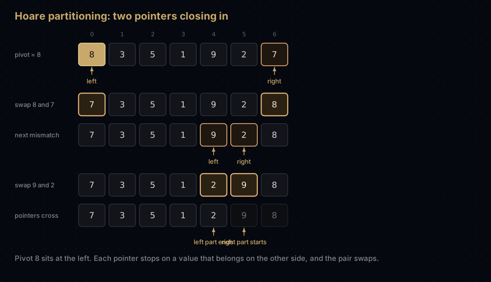
Hoare moves fewer elements, for a mechanical reason. Lomuto swaps once for every value that belongs on the left, about half of them on random data, and many of those swaps move a value onto itself. Hoare swaps only on a genuinely mismatched pair, one element on each wrong side, so on random data it does roughly half as many. Across 50 random lists of 200 integers, with the same median-of-three pivot for both, Lomuto's partitioning did about 38,000 swaps and Hoare's about 20,000.
Hoare is also far better on repeated values: both pointers stop on a value equal to the pivot, so equal elements end up spread across both sides. On 400 identical items Hoare needs 4,126 comparisons at depth 9; Lomuto needs 79,800 at depth 399, the full quadratic collapse, because every partition peels off one element. The price is that Hoare is easy to get wrong. Get the pivot position or the recursion bounds wrong and you get infinite recursion rather than a wrong answer.
How the code maps to the idea
partition is the entire algorithm; everything else is bookkeeping. The loop maintains one invariant: values[low:boundary + 1] holds values at most the pivot, and values[boundary + 1:scan] holds values greater than it. Each iteration either extends the second region by doing nothing, or extends the first by a slot and swaps the newcomer in. When the scan reaches high, the two regions cover everything but the pivot, so dropping the pivot at boundary + 1 finishes the job. The scan stops before high because high is the pivot itself; comparing it with itself would push the boundary one slot too far.
Both recursive calls exclude the pivot: split - 1 and split + 1, never split. That is what guarantees termination: every call gets a strictly shorter range than its parent. The base case, low >= high, covers an empty range and a single element at once, which is why the empty and one-item lists above need no special handling.
Quick sort is not stable. Partitioning swaps values across long distances, so two records that compare equal can come out in the opposite order to the one they went in. If you need stability, quick sort is the wrong tool, which is why Python's sorted() uses Timsort instead.
Choosing the pivot
Everything above used the last element as the pivot. That is the worst possible default, and here is the measurement. It counts comparisons and the depth of the recursion tree, using an explicit stack so a degenerate pivot cannot hit Python's recursion limit before the count finishes.
import random


def median_of_three(values: list[int], low: int, high: int) -> int:
    """Index of the median of the first, middle and last elements."""
    middle = (low + high) // 2
    first, centre, last = values[low], values[middle], values[high]

    if first <= centre <= last or last <= centre <= first:
        return middle
    if centre <= first <= last or last <= first <= centre:
        return low
    return high


def sort_with_stats(items: list[int], choose_pivot) -> tuple[int, int]:
    """Sort a copy and report (comparisons, depth of the recursion tree)."""
    values = list(items)
    comparisons = 0
    deepest = 0
    pending = [(0, len(values) - 1, 1)]

    while pending:
        low, high, depth = pending.pop()
        if low >= high:
            continue
        deepest = max(deepest, depth)

        # Move the chosen pivot to the end, then run the same Lomuto scan.
        chosen = choose_pivot(values, low, high)
        values[chosen], values[high] = values[high], values[chosen]

        pivot = values[high]
        boundary = low - 1
        for scan in range(low, high):
            comparisons += 1
            if values[scan] <= pivot:
                boundary += 1
                values[boundary], values[scan] = values[scan], values[boundary]
        values[boundary + 1], values[high] = values[high], values[boundary + 1]

        pending.append((low, boundary, depth + 1))
        pending.append((boundary + 2, high, depth + 1))

    assert values == sorted(items)
    return comparisons, deepest


def choose_last(values: list[int], low: int, high: int) -> int:
    return high


picker = random.Random(2024)


def choose_random(values: list[int], low: int, high: int) -> int:
    return picker.randrange(low, high + 1)


shuffler = random.Random(5)
ordered = list(range(400))
shuffled = [shuffler.randrange(1_000_000) for _ in range(400)]

print(f"{'pivot rule':<16}{'already sorted':>24}{'shuffled':>24}")
for name, rule in [("last element", choose_last),
                   ("median of three", median_of_three),
                   ("random", choose_random)]:
    sorted_cost, sorted_depth = sort_with_stats(ordered, rule)
    shuffled_cost, shuffled_depth = sort_with_stats(shuffled, rule)
    left = f"{sorted_cost} comps, depth {sorted_depth}"
    right = f"{shuffled_cost} comps, depth {shuffled_depth}"
    print(f"{name:<16}{left:>24}{right:>24}")

print("n(n-1)/2 =", 400 * 399 // 2)pivot rule already sorted shuffled
last element 79800 comps, depth 399 3602 comps, depth 18
median of three 2698 comps, depth 8 3017 comps, depth 13
random 3611 comps, depth 17 3558 comps, depth 17
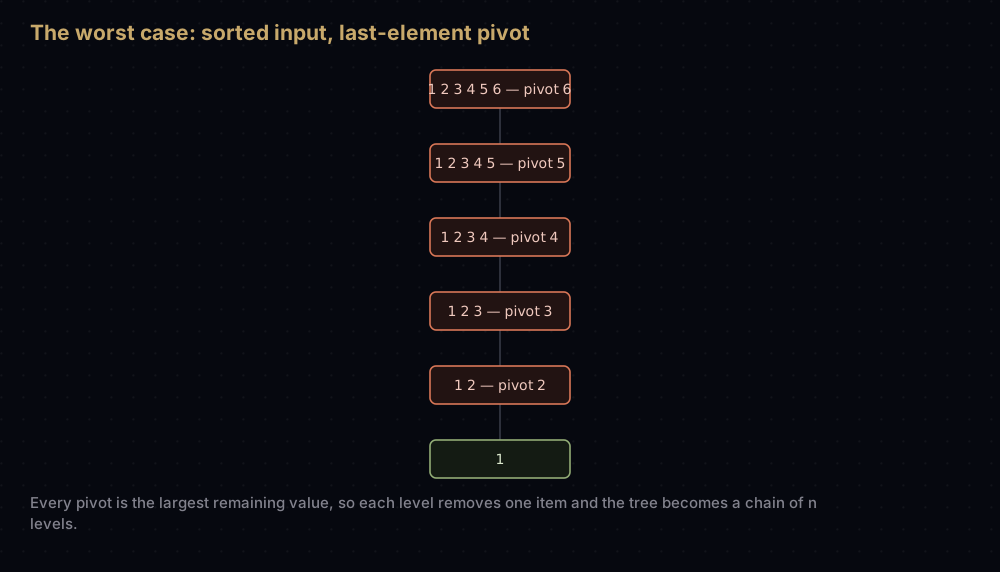
n(n-1)/2 = 79800Read the first row carefully. On already-sorted input the last-element pivot costs 79,800 comparisons at depth 399, and 79,800 is exactly n(n − 1) / 2 for n = 400, the same count as bubble sort. Sorted and reverse-sorted data is everywhere: database exports, log files, the output of an earlier sort. A first-or-last pivot means your sort is quadratic on the data it meets most often.
Two fixes, both cheap.
Median of three. Take the median of the first, middle and last elements. On sorted input the middle element is the true median, so the split is perfect. That is the 2,698 comparisons at depth 8 in the table, thirty times better on the same data. Three extra comparisons per partition turn both sorted and reverse-sorted input into the best case. It is what libstdc++ uses.
A random pivot. This does not remove the worst case — you could still draw the largest element every time — but it makes the worst case depend on your random numbers rather than on the input, so no particular input is bad and nobody who can see your data can construct a slow case for it.
Median of three is the usual production choice, being deterministic and best-case on the two commonest real patterns. Randomise when the input might be chosen by someone hostile.
Complexity
Every level of the recursion costs O(n). Partitioning a range of length m takes m − 1 comparisons, and the ranges at any one level are disjoint pieces of the original list, so all the partitions at one level together touch each element at most once. The only question left is how many levels there are.
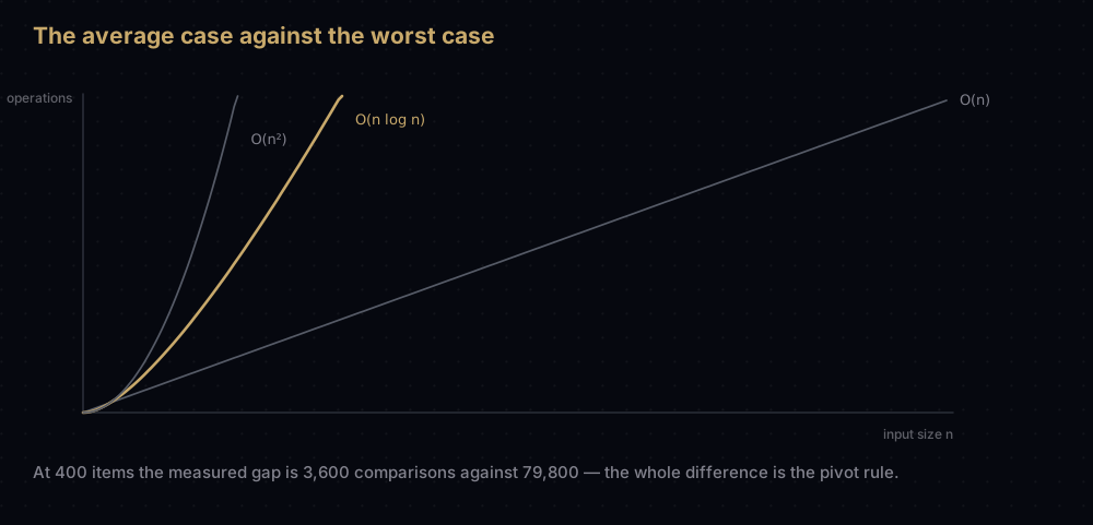
Best case: O(n log n). If every pivot lands in the middle, a range of length n becomes two of n/2, then four of n/4. After k levels the ranges have length n / 2^k, and they reach length 1 when k = log₂ n. That is log₂ n levels × O(n) per level = O(n log n).
Average case: O(n log n), with a constant near 1.39. This can be counted exactly rather than waved at. Take the two values that end up at ranks i and j in the sorted output. They are compared if and only if one of them is picked as a pivot while both are still in the same range: the moment any value ranked between them is picked, they are separated forever. There are j − i + 1 values in that rank window, each equally likely to be picked first, and exactly 2 of them cause a comparison, so the probability is 2 / (j − i + 1). Summing over every pair gives an expected 2(n + 1)Hₙ − 4n comparisons, where Hₙ is the harmonic number 1 + 1/2 + ... + 1/n. Hₙ grows like ln n, so that is about 2n ln n, or 1.39 n log₂ n, roughly 39% more comparisons than a perfectly balanced sort, and still O(n log n).
Check the formula against the random-pivot row above:
harmonic = sum(1 / k for k in range(1, 401))
print("predicted average:", round(2 * 401 * harmonic - 4 * 400))predicted average: 3669Predicted 3,669; measured 3,611 and 3,558 on the two inputs. The theory is not decoration.
That average is more robust than it looks. Suppose every partition were as lopsided as 10% / 90%. The longest chain of ranges then shrinks by a factor of 0.9 per level, and 0.9^k reaches 1/n at k = log n / log(10/9), about 6.6 log₂ n levels — still logarithmic. Quick sort breaks only when the splits are consistently extreme, not merely uneven.
Worst case: O(n²). The pivot is the smallest or largest value in the range every time, so one side is empty and the other holds n − 1 items. The levels shed one element each and there are n of them: (n − 1) + (n − 2) + ... + 1 = n(n − 1) / 2 comparisons. The first row of the table is exactly this.
Space: O(log n). The only memory beyond the list itself is the call stack, log₂ n frames deep when the splits are balanced. With bad splits a naive implementation recurses n deep and crashes: a real failure mode, not a theoretical one. The next section makes O(log n) a guarantee instead of an average.
The version you would actually ship
Three changes separate the teaching implementation from a real one.
Median-of-three pivots, as above. A cutoff for small ranges: below about 16 elements, insertion sort wins outright, because its inner loop is simpler and recursion stops paying for itself. Rather than sorting each small range separately, leave them and run one insertion sort over the whole array at the end: by then it is nearly sorted, so that pass is linear.
Recursion on the smaller side only. After partitioning, recurse into the shorter range and loop on the longer one by reassigning low or high. This is manual tail-call elimination, and it pins the stack down: the recursive call is always on at most half the current range, so after k nested calls the range is at most n / 2^k and the stack can never pass log₂ n frames — even while the sort itself runs in quadratic time.
CUTOFF = 16


def insertion_sort_range(values: list[int], low: int, high: int) -> None:
    """Insertion sort the slice values[low:high + 1] in place."""
    for index in range(low + 1, high + 1):
        current = values[index]
        position = index - 1
        while position >= low and values[position] > current:
            values[position + 1] = values[position]
            position -= 1
        values[position + 1] = current


def quick_sort_tuned(values: list[int]) -> None:
    """Quick sort with median-of-three pivots and a small-range cutoff."""
    tuned_sort_range(values, 0, len(values) - 1)
    insertion_sort_range(values, 0, len(values) - 1)


def tuned_sort_range(values: list[int], low: int, high: int) -> None:
    """Partition until every remaining range is short enough for insertion sort."""
    while high - low + 1 > CUTOFF:
        chosen = median_of_three(values, low, high)
        values[chosen], values[high] = values[high], values[chosen]
        split = partition(values, low, high)

        # Recurse into the smaller side, loop on the larger one, so the call
        # stack cannot grow past log2(n) frames however bad the pivots are.
        if split - low < high - split:
            tuned_sort_range(values, low, split - 1)
            low = split + 1
        else:
            tuned_sort_range(values, split + 1, high)
            high = split - 1


import sys

previous_limit = sys.getrecursionlimit()
sys.setrecursionlimit(100)

ascending = list(range(50_000))
quick_sort_tuned(ascending)
print("50,000 sorted items, recursion limit 100:", ascending == list(range(50_000)))

try:
    quick_sort(list(range(5_000)))
    print("the plain version survived")
except RecursionError:
    print("the plain version: RecursionError on the same input")

sys.setrecursionlimit(previous_limit)

checker = random.Random(11)
for _ in range(300):
    sample = [checker.randrange(30) for _ in range(checker.randrange(0, 80))]
    expected = sorted(sample)
    quick_sort_tuned(sample)
    assert sample == expected, sample
print("300 random lists sorted correctly")50,000 sorted items, recursion limit 100: True
the plain version: RecursionError on the same input
300 random lists sorted correctlyThe tuned version sorts 50,000 already-sorted items with Python's recursion limit dialled down to 100 frames. The plain version cannot manage 5,000 of them.
Real libraries add one more layer: introsort. Track the recursion depth, and if it passes 2 × log₂ n, abandon quick sort for that range and finish it with heap sort, which is O(n log n) no matter what. You keep quick sort's speed on normal data and inherit heap sort's guarantee on pathological data. That is what std::sort does in libstdc++ and libc++, and it is why the C++ standard can require O(n log n) worst case.
When to use it, and when not to
Use it when you are sorting values in memory, you do not need stability, and the extra O(n) array merge sort wants is unwelcome. It beats merge sort on real machines despite the worse bound for three reasons: no allocation, an inner loop that scans contiguous memory with near-perfect cache locality, and very little work per comparison.
Do not use it when you need stability, when a quadratic outlier is a safety problem rather than an annoyance, or when the data is on disk. Sorting records by one field and expecting ties to keep their previous order needs merge sort or Timsort. Hard real-time code should use heap sort (O(n log n) always, in place), or introsort. A file larger than memory is merge sort's territory, because merging is sequential and partitioning is not.
In Python, do not write it at all. sorted(items) and items.sort() run Timsort in C: O(n log n) worst case, stable, adaptive to partly ordered data, and an order of magnitude faster than anything you write in Python itself. Learn quick sort to understand what libraries do, not to use it here.
Where it shows up in the real world
C++'s std::sort is introsort. libstdc++ is the clearest example: quick sort with median-of-three pivots, a switch to heap sort past a recursion depth of 2 × log₂ n, and a final insertion-sort pass over ranges shorter than 16: the three refinements built above. libc++ has the same shape with different constants.
Java's Arrays.sort on primitive arrays uses dual-pivot quick sort, partitioning into three regions around two pivots at once. Java's object sort is TimSort instead, because sorting objects has to be stable.
Go's slices.Sort and Rust's slice::sort_unstable use pattern-defeating quicksort or a direct descendant of it: a variant that detects the patterns which make ordinary quick sort quadratic (sorted runs, many equal keys), and handles them in linear time.
Quickselect is the partition step on its own. To find the k-th smallest value, partition once, see which side k falls in, and recurse into that side only. Discarding half the data each time instead of processing both halves costs n + n/2 + n/4 + ... = O(n) expected — a median without sorting. The worst case is still quadratic, for exactly the reason quick sort's is, which is why NumPy's np.partition and np.median run introselect: quickselect with a fallback that pins the bound at linear.
Python's sorted() is the honest counterexample. It does not use quick sort, for the two weaknesses above: Python guarantees a stable sort, and Timsort's adaptivity to already-ordered runs beats quick sort on partly sorted data.
Common mistakes
Recursing on the pivot's own index. With Lomuto you must pass split - 1 and split + 1. Including split means the range never shrinks, and [2, 2] recurses until the stack dies.
Mixing the two schemes. Hoare's loop with pivot = values[high] is the classic trap: the returned index can equal high, so one recursive call gets the whole range back and never terminates. Hoare needs the pivot at low or the midpoint and includes split on the left; Lomuto needs it at high and excludes split. Never half-convert one into the other.
Choosing median-of-three and forgetting to move it. median_of_three returns an index; partition requires the pivot to be sitting at high. Skip the swap between them and you have chosen a pivot the partition never uses.
Assuming duplicates are harmless. Lomuto's values[scan] <= pivot sends every equal value left, so identical items partition into n − 1 and 0 every time: 79,800 comparisons for 400 items. With many repeated keys, use three-way partitioning (the Dutch national flag scheme, which splits into less-than, equal-to and greater-than and never recurses into the equal block), or switch to Hoare.
Trusting the average on untrusted input. A fixed pivot rule can be driven quadratic on purpose; McIlroy's 1999 paper "A Killer Adversary for Quicksort" builds such an input for any deterministic comparison-based implementation. If the data comes from users, randomise the pivot or add the introsort depth limit.
Practice
- Add a
descending: bool = Falseparameter topartition, changing only the comparison. - Write
quickselect(values, k), returning the k-th smallest value by recursing into one side of the partition only, and check it againstsorted(values)[k]. - Implement three-way partitioning and compare its comparison count with Lomuto's on 1,000 items drawn from five distinct values.
- Add a depth budget of 2 × log₂ n to
tuned_sort_rangeand fall back toheapqwhen it runs out: introsort in about six lines. - Record the size of every range the sort partitions, and confirm the sizes at each level of the tree sum to at most n.
Summary
Quick sort is a partition-and-recurse sort with an O(n²) worst case that almost never happens and an O(n log n) average that beats every other comparison sort on real hardware. The difference between those outcomes is the pivot rule: median-of-three or a random index turns the common bad inputs into ordinary ones, and smaller-side recursion holds the stack at log₂ n frames regardless.
| Difficulty | Medium |
| Best case | O(n log n) — balanced splits, log₂ n levels of O(n) work |
| Average case | O(n log n) — expected 2n ln n ≈ 1.39 n log₂ n comparisons |
| Worst case | O(n²) — extreme pivot every time, n(n − 1) / 2 comparisons |
| Space | O(log n) — call stack only, with smaller-side recursion |
| Stable | No — partitioning swaps equal values across the list |
| In place | Yes |
| Adaptive | No — sorted input is the worst case unless the pivot rule fixes it |
| Data structure | List / array with O(1) indexing |
| Use it when | Sorting in memory, stability not needed, memory is tight |
| Avoid it when | You need stability, a hard worst-case bound, or you sort on disk |
| Real-world use | std::sort (introsort), Java's primitive Arrays.sort, Go's slices.Sort |
| Python equivalent | sorted(items) / items.sort() — Timsort, stable, O(n log n) worst case |
Write it once from memory, pivot choice and smaller-side recursion included. Then reach for sorted().
Keep reading
- Merge Sort in Python — the same divide-and-conquer shape with the work done coming back up, and a worst case that never degrades.
- Heap Sort in Python — the O(n log n) guarantee introsort escapes to when quick sort goes bad.
- Insertion Sort in Python — the small-range sort every tuned quick sort finishes with.
- Timsort — what
sorted()actually runs, and why Python chose stability instead. - Big O Notation — the counting arguments behind every bound above.


