Selection sort writes to the array 2(n − 1) times and no more, whatever you feed it. Hand it 1,000 items in reverse order and it performs 1,998 element writes. Bubble sort, given the same list, performs 999,000. That is not a better average. It is a hard ceiling no input can push past, and no other simple sort has one anywhere near it.
Everything else about it is worse than the alternatives. It is not stable, it is not adaptive, and it makes exactly the same n(n − 1) / 2 comparisons whether you give it a sorted list, a shuffled one or a reversed one. Insertion sort beats it on almost every realistic input.
Learn it anyway, for two reasons. The bounded write count is the right property when a write is expensive: flash and EEPROM cells wear out after a finite number of writes, and it is the writes that kill them. And selection sort is heap sort with the clever part missing: swap its linear scan for a binary heap and the O(n²) becomes O(n log n), the cleanest example in this series of a data structure turning into a speedup.
The idea
Split the list into two regions: a sorted prefix on the left, which starts empty, and an unsorted region on the right, which starts as the whole list. The boundary between them is a single index.
Then repeat one step until the unsorted region has one item left in it:
- Scan the whole unsorted region and find the smallest value in it.
- Swap that value with whatever is sitting at the very front of the unsorted region.
- Move the boundary one place right.
The value you just placed is now part of the sorted prefix, and it never moves again.
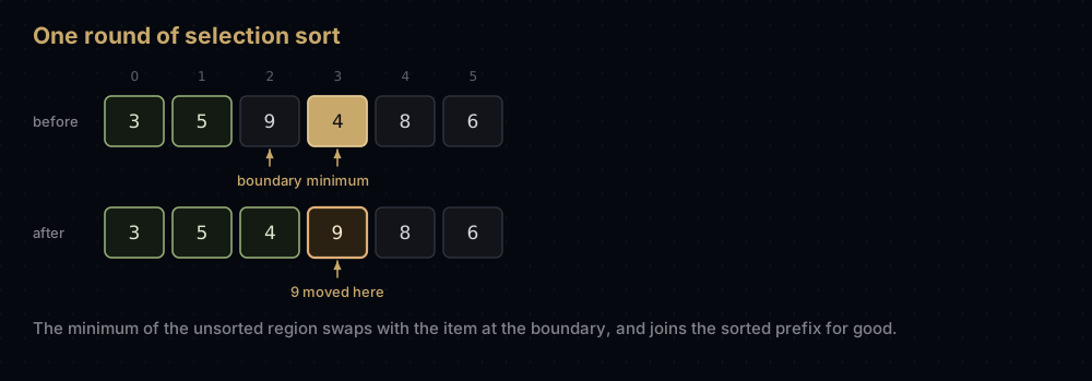
Why that prefix must be correct is the whole proof. Each round selects the minimum of everything that is left, so the value placed in round two was chosen from a set that still contained every value placed later, and is no larger than any of them. Repeat, and the prefix comes out in non-decreasing order with every entry in its final position.
Compare bubble sort, which moves a value one position per swap. Selection sort sends a value straight home in one jump, and pays for it with a full scan of the remaining region.
Watching it work
Take the list [29, 10, 14, 37, 13]. Five items, so four rounds.
Round 1 — the region is the whole list. Assume the first item, 29, is the smallest, then check the rest. 10 beats 29, so the running minimum becomes 10 at index 1; 14, 37 and 13 all lose to it. Swap indices 0 and 1: [10, 29, 14, 37, 13], and index 0 is finished. Four comparisons.
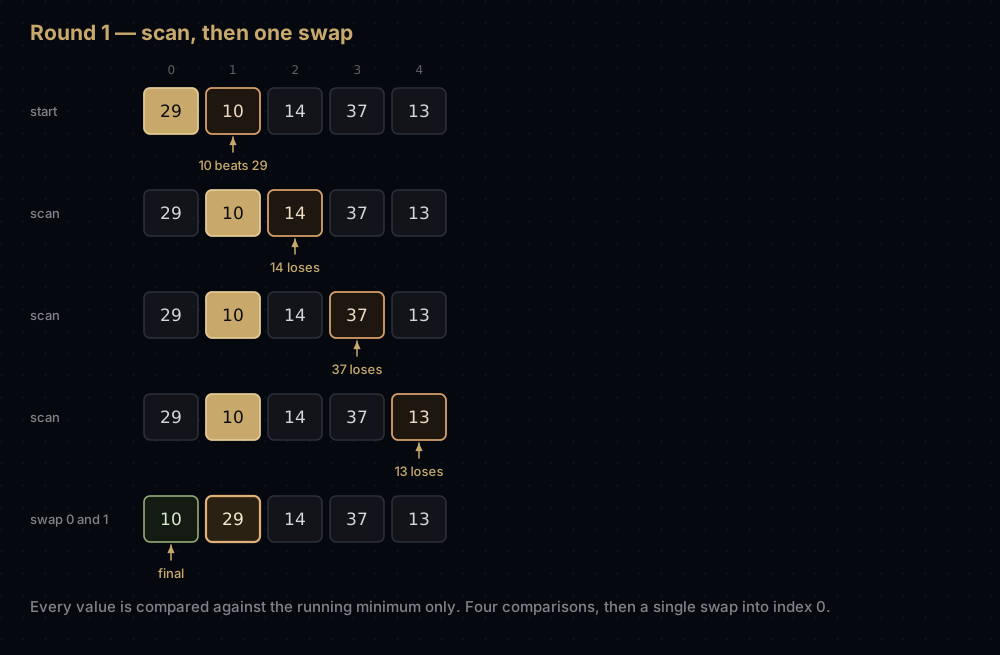
Round 2 — region 29, 14, 37, 13. The running minimum drops from 29 to 14 to 13 at index 4. Swap indices 1 and 4: [10, 13, 14, 37, 29]. Three comparisons.
Round 3 — region 14, 37, 29. The minimum 14 is already at index 2, so the code swaps index 2 with itself and moves on. Two comparisons.
Round 4 — region 37, 29. The minimum is 29 at index 4. Swap: [10, 13, 14, 29, 37]. One comparison.
One item is left, and a single item has nowhere else to be. Total: 4 + 3 + 2 + 1 = 10 comparisons and 4 swaps, one of which moved nothing.
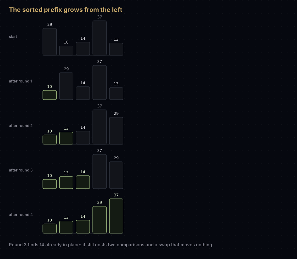
Round 3 is the one to stare at. It scanned three values, found the minimum already in place, performed a swap that moved nothing, and still charged two comparisons. Selection sort cannot skip it, because it has no way to know in advance. That is the whole reason it has no best case.
The code
def selection_sort(items: list[int]) -> list[int]:
    """Sort ascending by repeatedly moving the smallest unsorted value forward.

    Sorts a copy, so the caller's list is untouched. Drop the copy and return
    None to sort genuinely in place.
    """
    values = list(items)
    n = len(values)

    for boundary in range(n - 1):
        # Everything before `boundary` is already final. Find the smallest
        # value in what remains, then put it at `boundary`.
        minimum_index = boundary
        for index in range(boundary + 1, n):
            if values[index] < values[minimum_index]:
                minimum_index = index

        values[boundary], values[minimum_index] = values[minimum_index], values[boundary]

    return values


print(selection_sort([29, 10, 14, 37, 13]))
print(selection_sort([]))
print(selection_sort([3]))
print(selection_sort([2, 2, 1]))[10, 13, 14, 29, 37]
[]
[3]
[1, 2, 2]That is the complete algorithm. Unlike bubble sort there is no optimised second version, because there is no boolean you can add to make it faster.
How the code maps to the idea
boundary is the split. Indices 0 to boundary - 1 are the sorted prefix; boundary to n - 1 are the unsorted region. The outer loop walks the boundary rightwards.
The outer loop stops at n - 1, not n. Once n − 1 items are placed, the one left over must be the largest: everything smaller was extracted earlier. A final round would compare nothing and swap that item with itself.
minimum_index tracks an index, not a value. You need the position in order to swap. Seeding it with boundary rather than float("inf") also keeps the code working on any comparable type.
The inner loop starts at boundary + 1. Starting at boundary merely wastes a comparison of an item against itself. Starting at 0 is a real bug: see the mistakes section.
The comparison is strictly <. On a tie minimum_index does not move, so the earliest of several equal values wins the scan. That is the right choice, and still not enough to make the algorithm stable: the swap is what ruins that.
Edge cases fall out of the arithmetic. An empty list gives range(-1) and a one-item list range(0); both are empty, so nothing runs and neither needs a special case.
Why it is not stable
A sort is stable if two items that compare equal come out in the same relative order they went in. That is what lets you sort a table by date, then by name, and still have each name's rows in date order.
Selection sort is not stable, and the counterexample is tiny: three records scored 2, 2 and 1.
def selection_sort_by_score(records: list[tuple[str, int]]) -> list[tuple[str, int]]:
    """Selection sort on (name, score) pairs, ordering by score only."""
    values = list(records)
    n = len(values)

    for boundary in range(n - 1):
        minimum_index = boundary
        for index in range(boundary + 1, n):
            if values[index][1] < values[minimum_index][1]:
                minimum_index = index
        values[boundary], values[minimum_index] = values[minimum_index], values[boundary]

    return values


scores = [("ana", 2), ("ben", 2), ("cy", 1)]
print(selection_sort_by_score(scores))
print(sorted(scores, key=lambda record: record[1]))[('cy', 1), ('ben', 2), ('ana', 2)]
[('cy', 1), ('ana', 2), ('ben', 2)]ana went in before ben and came out after it. Python's built-in sorted, which is stable, keeps them in input order.
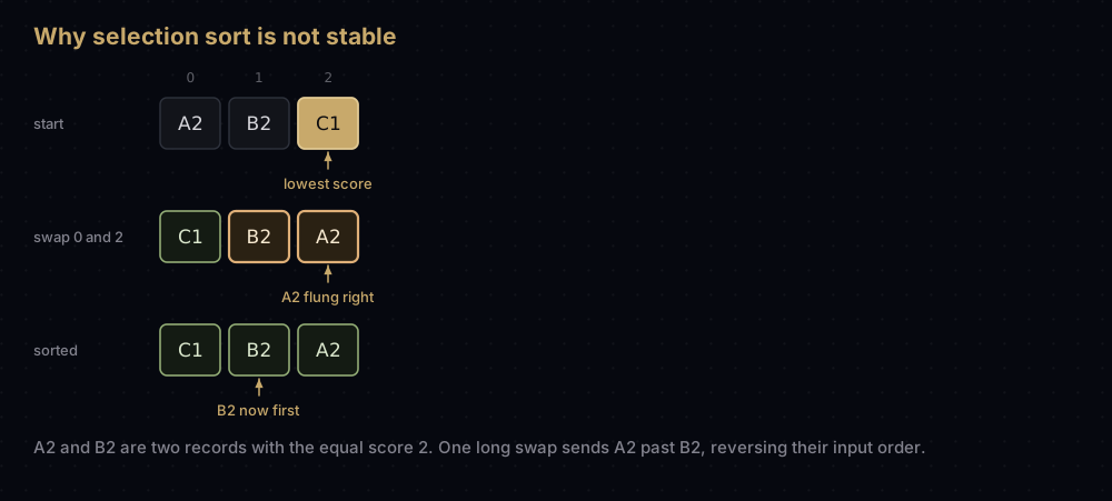
The mechanism is easy to see. Round 1 finds the minimum, cy, at index 2 and swaps it with index 0, which does not just move cy left, it flings ana out to index 2, right over ben. Any sort that moves an element a long distance in one step risks jumping it across an equal key. Bubble and insertion sort only ever move things one slot past a strictly larger neighbour, which is why they get stability for free.
You can make it stable, at the cost of the thing that made it interesting: instead of swapping, shift the whole block right by one and drop the minimum into the gap.
def stable_selection_sort(records: list[tuple[str, int]]) -> list[tuple[str, int]]:
    """Selection sort made stable by rotating the minimum into place.

    Instead of swapping the minimum with the boundary element, everything
    between them shifts one slot right. Equal keys keep their input order,
    but the write count climbs back to O(n^2).
    """
    values = list(records)
    n = len(values)

    for boundary in range(n - 1):
        minimum_index = boundary
        for index in range(boundary + 1, n):
            if values[index][1] < values[minimum_index][1]:
                minimum_index = index

        minimum = values[minimum_index]
        # Shifting preserves the relative order of everything passed over,
        # which is exactly what the long-distance swap destroyed.
        for index in range(minimum_index, boundary, -1):
            values[index] = values[index - 1]
        values[boundary] = minimum

    return values


print(stable_selection_sort(scores))[('cy', 1), ('ana', 2), ('ben', 2)]Stable — and now doing up to n(n + 1) / 2 − 1 writes instead of 2(n − 1). If you want that trade you have just described insertion sort, which does the same shifting with far fewer comparisons.
Why it is not adaptive
An adaptive sort runs faster on input that is already partly ordered. Bubble sort becomes adaptive with one boolean: a pass that performs no swaps proves every adjacent pair is in order, which proves the list is sorted.
Selection sort has no equivalent, for a structural reason. Its scan only ever compares a candidate against the running minimum, never two candidates against each other. When the round ends you know exactly one fact, which value is smallest, and nothing about how the rest are ordered. There is no certificate to collect.
The tempting bug is to copy bubble sort's flag anyway and stop when a round makes no swap. [1, 3, 2] breaks that: round 1 finds 1 already at index 0, swaps nothing, and the early exit hands back an unsorted list.
So the comparison count is fixed by the length of the list alone:
def selection_sort_counted(items: list[int]) -> tuple[list[int], int, int]:
    """Same algorithm, also reporting comparisons and swaps performed."""
    values = list(items)
    n = len(values)
    comparisons = swaps = 0

    for boundary in range(n - 1):
        minimum_index = boundary
        for index in range(boundary + 1, n):
            comparisons += 1
            if values[index] < values[minimum_index]:
                minimum_index = index
        values[boundary], values[minimum_index] = values[minimum_index], values[boundary]
        swaps += 1

    return values, comparisons, swaps


for label, data in [
    ("sorted  ", [1, 2, 3, 4, 5, 6, 7, 8]),
    ("reversed", [8, 7, 6, 5, 4, 3, 2, 1]),
    ("shuffled", [5, 3, 8, 1, 7, 2, 6, 4]),
]:
    _, comparisons, swaps = selection_sort_counted(data)
print(f"{label} {comparisons} comparisons, {swaps} swaps")sorted 28 comparisons, 7 swaps
reversed 28 comparisons, 7 swaps
shuffled 28 comparisons, 7 swapsThree completely different inputs, identical work. Bubble sort on those same lists ranges from 7 comparisons to 28.
Complexity
Comparisons: always n(n − 1) / 2
Round 1 compares the running minimum against n − 1 candidates, round 2 against n − 2, and the region shrinks by one each time down to a final round with 1 comparison:
(n − 1) + (n − 2) + … + 2 + 1 = n(n − 1) / 2
Multiply out and that is (n² − n) / 2. Big O discards the constant ½ and the smaller −n term, leaving O(n²).
The important word is always. Both loop bounds are computed from n and boundary; neither reads the data, so no arrangement of values can make the inner loop run fewer times. Best, average and worst case are all Θ(n²): pinned from both directions, not merely bounded above. The n = 8 run confirms it: 8 × 7 / 2 = 28, every time.
Writes: always 2(n − 1)
Each round performs exactly one swap and there are n − 1 rounds, so there are n − 1 swaps and 2(n − 1) element writes, on every input including the reversed one. That is O(n) writes — linear, not quadratic.
No other simple sort has a worst case anywhere near it. Bubble sort swaps once per inversion, and a reversed list of n items has n(n − 1) / 2 inversions, so it writes n(n − 1) times. Insertion sort shifts once per inversion too. Here is the gap at n = 1,000:
def bubble_sort_writes(items: list[int]) -> int:
    """Count the element writes a bubble sort performs: two per swap."""
    values = list(items)
    n = len(values)
    writes = 0

    for pass_number in range(n - 1):
        swapped = False
        for index in range(n - 1 - pass_number):
            if values[index] > values[index + 1]:
                values[index], values[index + 1] = values[index + 1], values[index]
                writes += 2
                swapped = True
        if not swapped:
            break

    return writes


reversed_thousand = list(range(1000, 0, -1))
_, _, selection_swaps = selection_sort_counted(reversed_thousand)

print("bubble sort writes   :", bubble_sort_writes(reversed_thousand))
print("selection sort writes:", 2 * selection_swaps)bubble sort writes : 999000
selection sort writes: 1998Five hundred times fewer writes, for the same n² comparisons. One honest footnote: some of those swaps put an element back onto itself, as round 3 did above. Guarding with if minimum_index != boundary turns "exactly n − 1 swaps" into "at most n − 1" and skips the wasted writes. The bound does not change; the constant improves.
The honesty runs the other way at the easy end. Give all three sorts a list of 1,000 items that is already in order: bubble sort's early exit writes nothing at all, insertion sort writes 999, and selection sort still performs its full 1,998. The ceiling is what selection sort wins on, not every individual input.
Space: O(1)
Two integers, boundary and minimum_index, however big the list is, and the swap happens inside the array. The version above returns a copy for convenience, costing O(n): delete the list(items) call and it sorts in place with genuinely constant extra space.
The two costs in absolute numbers
| Items | Comparisons, every input | Element writes |
|---|---|---|
| 10 | 45 | 18 |
| 100 | 4,950 | 198 |
| 1,000 | 499,500 | 1,998 |
| 10,000 | 49,995,000 | 19,998 |
| 100,000 | 4,999,950,000 | 199,998 |
Ten times the data costs a hundred times the comparisons but only ten times the writes. The two columns grow at completely different rates, and that difference is the entire case for this algorithm.
When to use it, and when not to
Use it when a write costs far more than a comparison. That is the one scenario where it wins on merit rather than on simplicity. If comparisons are cheap register operations and each write is an erase-and-program cycle on memory that wears out, trading n² comparisons for 2n writes is the correct engineering call.
Use it when n is tiny and you want code you can write correctly from memory. Under about 20 items the choice of sorting algorithm disappears into the noise.
Avoid it everywhere else. In Python, sorting is sorted(items) or items.sort(), which run Timsort: a stable, adaptive, O(n log n) hybrid implemented in C. If you want a simple hand-written sort, insertion sort is strictly better: same code size, stable, and O(n) on nearly-sorted input where selection sort still grinds through its full n(n − 1) / 2.
Do not reach for it just to get the smallest few items. Running only k rounds yields the k smallest in O(nk), but heapq.nsmallest(k, items) does that job in O(n log k), and min(items) is the k = 1 case.
Selection sort and heap sort are the same algorithm
Strip selection sort down to its skeleton and you get this:
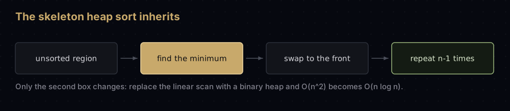
Every part of that skeleton is already optimal except step two. Finding the minimum by scanning costs O(n) and you do it n times, which is exactly where the n² comes from. You cannot make a linear scan faster, but you can stop scanning: keep the unsorted region in a binary heap, a tree-shaped arrangement that hands you its smallest element in O(1) and repairs itself in O(log n) after you remove it.
The outer loop is then unchanged (still n rounds, one extraction and one placement each), but a round costs O(log n) instead of O(n), for O(n log n) overall. That algorithm is heap sort. Real implementations mirror it, using a max-heap and growing the sorted region from the right so the heap and the output can share one array, but the skeleton is the same. So are the family traits: heap sort is in place, not stable and not adaptive, for the same reasons selection sort is not.
Where it shows up in the real world
No mainstream standard library, database or language runtime sorts with selection sort. As with bubble sort, that is a deliberate omission rather than an oversight.
Its legitimate niche is write-limited storage. EEPROM and flash cells do not last forever: an EEPROM cell is typically rated for 100,000 to 1,000,000 program/erase cycles, the NOR flash inside a microcontroller often for around 10,000, and multi-level NAND flash lower still. Firmware that reorders a table stored directly in such memory is in the rare position where the write count, not the comparison count, decides whether the hardware survives. A flat 2(n − 1) writes is the right shape for that.
Be honest about the limits of that argument. If the table fits in RAM — and on any device with more than a few kilobytes it does — read it out, sort it in RAM, and write it back once. That is n writes, beating every in-place scheme. And if you genuinely need the fewest possible writes, cycle sort achieves the provable minimum: each element written at most once, in exchange for O(n²) comparisons and fiddlier code.
The second real property is predictability: identical work for every input of a given size. In a hard real-time loop, where you budget for the worst case anyway, an algorithm whose worst case equals its average case is easier to reason about, though quadratic and predictable is still quadratic, so this only helps at small fixed n.
Beyond that its job is educational: the shortest route to understanding heap sort, and the clearest demonstration that comparisons and writes are separate costs you can trade against each other.
Common mistakes
Scanning from index 0 instead of the boundary. With for index in range(n) the scan re-examines the sorted prefix. From round 2 onwards the global minimum sits at index 0, already placed, so minimum_index comes back as 0 and the code drags a finished element back into the unsorted region. The result is not sorted.
Tracking the smallest value instead of its index. You reach the end of the scan holding 13 and no idea where it lives, so you cannot swap it. Track minimum_index and read values[minimum_index] when you need the value.
Swapping inside the inner loop. if values[index] < values[boundary]: swap(boundary, index) still produces a sorted list, so it survives your tests. It also performs up to n(n − 1) / 2 swaps instead of n − 1, throwing away the only reason to choose this algorithm.
Adding bubble sort's early-exit flag. A round that swaps nothing only tells you the smallest remaining value happened to be at the front. On [1, 3, 2] that exit fires immediately and returns the list unsorted.
Assuming it is stable because it swaps so rarely. Each rare swap can travel the length of the array, which is precisely what breaks stability. To sort records by a secondary key, use sorted(records, key=...).
Using <= instead of < in the scan. It still sorts, but moves minimum_index on every tie for no benefit, and it would break the stable shifting variant by selecting the last equal key rather than the first.
Practice
- Rewrite
selection_sortto sort the caller's list in place and returnNone, then confirm the original list really changed. - Change it to select the maximum each round and place it at the end of the unsorted region, and check it still produces ascending output.
- Write
k_smallest(items, k)that runs only k rounds, and compare its results withheapq.nsmallest(k, items). - Implement double selection sort: find the minimum and maximum in one scan and place both, halving the rounds. Count its comparisons and work out whether it really beats n(n − 1) / 2.
- Implement cycle sort and count its element writes on a reversed list of 20 items. Selection sort uses 38 there: see how far below that you can get.
Summary
Selection sort is the one simple sort with a linear write count, and that is the only reason to pick it. Everything else is a step backwards: no stability, no adaptivity, and a comparison count nailed to n(n − 1) / 2 whatever the input. The real reward for learning it is structural. It is heap sort with the heap taken out, which makes the jump to O(n log n) feel inevitable rather than magical.
| Difficulty | Easy |
| Best case | O(n²) — the scan length never depends on the data |
| Average case | O(n²) — n(n − 1) / 2 comparisons, on every input |
| Worst case | O(n²) — identical to the best case |
| Space | O(1) — two index variables, swaps in place |
| Element writes | O(n) — exactly 2(n − 1), the lowest worst case of any simple sort |
| Stable | No — the long swap jumps one equal key over another |
| In place | Yes |
| Adaptive | No — a round collects no evidence about the rest of the list |
| Data structure | List / array with O(1) indexing |
| Use it when | Writes cost far more than comparisons, or n is under ~20 |
| Avoid it when | Anything else — insertion sort is faster and stable |
| Real-world use | None in mainstream libraries; a fit for write-limited memory, and the ancestor of heap sort |
| Python equivalent | sorted(items) / items.sort(); heapq.nsmallest(k, items) for the k smallest |
Keep reading
- Heap Sort in Python — this skeleton with a heap in the middle, and the O(n log n) that falls out.
- Insertion Sort in Python — the simple sort actually worth using, and the one that beats this on nearly-sorted data.
- Bubble Sort in Python — the other O(n²) classic, and the adaptive counterpart to this one.
- Heaps and Priority Queues in Python — the structure that makes "give me the smallest" cost O(log n).
- Big O Notation — the counting arguments used above, in full.


