Looking up a name in a phone book with a million entries does not take a million checks. It takes twenty. Open it near the middle, see whether the name you want falls before or after that page, and throw away the half it cannot possibly be in. Repeat on what is left. Twenty is not a guess: you can only halve a million about twenty times before nothing remains.
That is binary search, and it buys its speed with a precondition. The data must already be sorted, and you must be able to jump straight to the middle item without walking there. A Python list gives you that jump for free. A linked list, a generator, or a file you are reading line by line does not, and binary search is simply unavailable there.
It is also the algorithm people get wrong most often. Jon Bentley, in Programming Pearls, gave professional programmers at Bell Labs and IBM a couple of hours to write a binary search from a plain-English description; only about ten percent produced a correct one. Every failure lives in the boundaries, which index the middle is, whether the window includes its endpoints, and whether the next window actually got smaller. So this post nails the boundaries down, counts where the logarithm comes from, shows the standard-library version you should use at work, and then reuses the same halving on a problem that has no list in it at all.
The idea
You have a sorted list and a target. Keep track of a window: the stretch of the list the target could still be in. It starts as the whole list.
Look at the item in the middle of the window and compare it to your target. Exactly one of three things is true:
- It equals the target. You are done.
- It is smaller than the target. Since the list is sorted, every item to its left is smaller too, so the target cannot be there. Move the window's left edge to just past the middle.
- It is larger than the target. Symmetrically, everything to its right is larger, so the target cannot be there. Move the window's right edge to just before the middle.
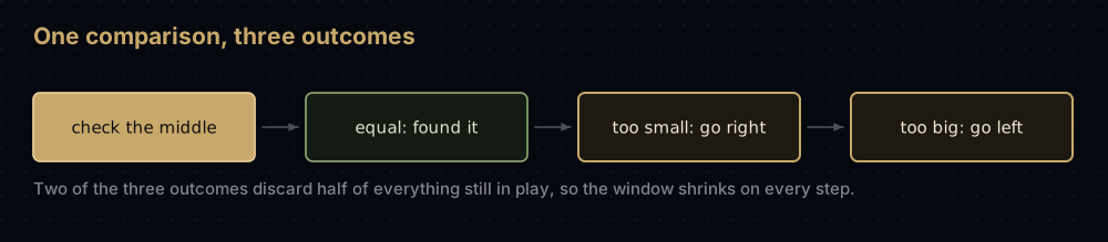
Repeat until the target turns up or the window becomes empty. An empty window is a proof of absence, not a failure to look hard enough: every item ever discarded was ruled out by a comparison.
The sorted precondition is what makes the second and third deductions legal. On unsorted data those deductions are false, so binary search does not merely run slower: it returns wrong answers, quietly, and it returns them fast.
Watching it work
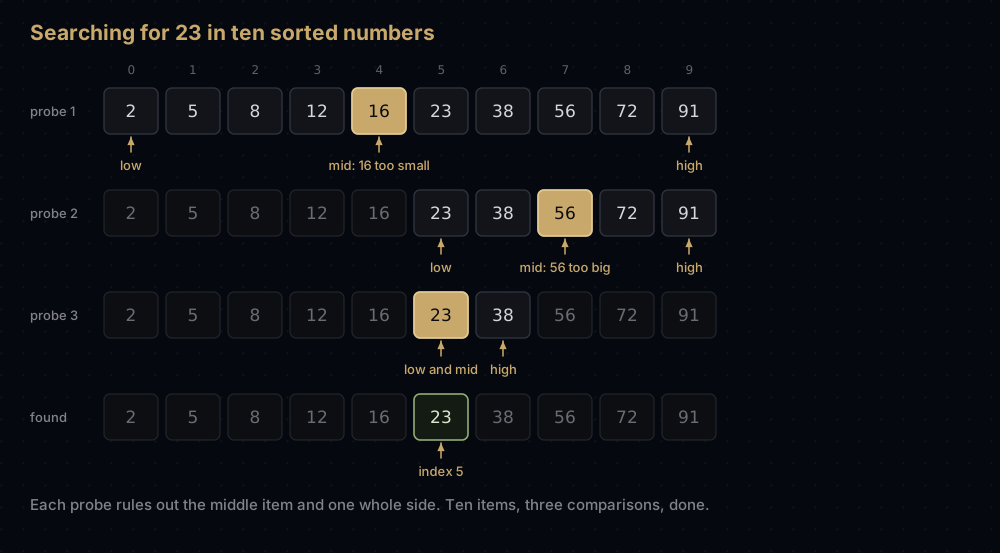
Take this sorted list of ten numbers and search for 23.
index    0   1   2    3    4    5    6    7    8    9
value    2   5   8   12   16   23   38   56   72   91
Probe 1. The window is the whole list, low = 0 and high = 9. The middle index is 0 + (9 - 0) // 2 = 4, holding 16. Since 16 < 23, everything at index 4 and below is out. Set low = 5.
Probe 2. The window is indices 5 to 9. The middle index is 5 + (9 - 5) // 2 = 7, holding 56. Since 56 > 23, index 7 and everything above is out. Set high = 6.
Probe 3. The window is indices 5 to 6, just 23 and 38. The middle index is 5 + (6 - 5) // 2 = 5, holding 23. Found, at index 5, after three comparisons. A linear scan would have taken six.
Now search for 40, which is not in the list. Probes 1 and 2 go exactly as before. Probe 3 looks at 23, which is smaller than 40, so low = 6. Probe 4 has a one-item window holding 38, which is also smaller, so low = 7. Now low is 7 and high is 6: the window is empty, and the algorithm reports absence after four probes.
Notice what "empty window" means here. low = 7 and high = 6 says the target belongs between index 6 and index 7, which is exactly the information bisect returns later in this post, and it is more useful than a bare "not found".
The code
Here is the iterative version. It is the one to memorise.
def binary_search(items: list[int], target: int) -> int:
    """Return the index of target in a sorted list, or -1 if it is absent.

    items must already be in ascending order. Given unsorted input the
    function does not complain, it just returns a wrong answer.
    """
    low, high = 0, len(items) - 1

    while low <= high:
        # low + (high - low) // 2 rather than (low + high) // 2: the two agree
        # in Python, but only the first is safe in a fixed-width language.
        middle = low + (high - low) // 2
        guess = items[middle]

        if guess == target:
            return middle
        if guess < target:
            low = middle + 1      # everything up to middle is too small
        else:
            high = middle - 1     # everything from middle on is too large

    return -1


numbers = [2, 5, 8, 12, 16, 23, 38, 56, 72, 91]
print(binary_search(numbers, 23))
print(binary_search(numbers, 2))
print(binary_search(numbers, 91))
print(binary_search(numbers, 40))
print(binary_search([], 40))5
0
9
-1
-1The same function, printing its window at every step, so you can check the walkthrough above against what the machine actually does:
def binary_search_traced(items: list[int], target: int) -> int:
    """Binary search that reports the window it is left with after each probe."""
    low, high = 0, len(items) - 1
    probes = 0

    while low <= high:
        middle = low + (high - low) // 2
        probes += 1
        print(f"probe {probes}: window {items[low:high + 1]}, "
              f"middle index {middle} holds {items[middle]}")

        if items[middle] == target:
            print(f"found {target} at index {middle} after {probes} probes")
            return middle
        if items[middle] < target:
            low = middle + 1
        else:
            high = middle - 1

    print(f"{target} is absent, and {probes} probes were enough to prove it")
    return -1


binary_search_traced(numbers, 23)
print()
binary_search_traced(numbers, 40)probe 1: window [2, 5, 8, 12, 16, 23, 38, 56, 72, 91], middle index 4 holds 16
probe 2: window [23, 38, 56, 72, 91], middle index 7 holds 56
probe 3: window [23, 38], middle index 5 holds 23
found 23 at index 5 after 3 probes
probe 1: window [2, 5, 8, 12, 16, 23, 38, 56, 72, 91], middle index 4 holds 16
probe 2: window [23, 38, 56, 72, 91], middle index 7 holds 56
probe 3: window [23, 38], middle index 5 holds 23
probe 4: window [38], middle index 6 holds 38
40 is absent, and 4 probes were enough to prove itThe recursive form says the same thing differently: searching a window is the same problem as searching a smaller window.
def search_between(items: list[int], target: int, low: int, high: int) -> int:
    """Search items[low:high + 1] only. An empty window means the target is absent."""
    if low > high:
        return -1

    middle = low + (high - low) // 2
    if items[middle] == target:
        return middle
    if items[middle] < target:
        return search_between(items, target, middle + 1, high)
    return search_between(items, target, low, middle - 1)


def binary_search_recursive(items: list[int], target: int) -> int:
    """The same halving, expressed as a smaller copy of the same problem."""
    return search_between(items, target, 0, len(items) - 1)


print([binary_search_recursive(numbers, value) for value in numbers])
print(binary_search_recursive(numbers, 40))[0, 1, 2, 3, 4, 5, 6, 7, 8, 9]
-1Prefer the iterative one. The recursion is not doing any bookkeeping a loop cannot do, each call costs a stack frame, and Python does not optimise tail calls. The depth is only about log₂ n, so it will never blow the stack on real data, but you gain nothing for the frames.
How the code maps to the idea
The window is low to high inclusive. Both endpoints are live candidates. That single decision fixes everything else: the loop condition is low <= high (a window of one item is still a window worth checking), and an empty window is the moment low overtakes high.
middle is the floor of the halfway point. With low = 5 and high = 6, middle is 5, not 5.5 and not 6. Integer division always rounds down, so middle can equal low but never equals high unless the window holds a single item. That rounding is why low = middle is the classic hang: on a two-item window it changes nothing at all.
The two updates use middle + 1 and middle - 1, never plain middle. You already compared items[middle] and it was not the target, so it belongs in neither half. Excluding it is what guarantees the window shrinks by at least one item per probe, and that guarantee is the whole termination argument. Write low = middle instead and the code hangs forever on the right input:
def broken_search(items: list[int], target: int, step_limit: int = 5) -> int:
    """The classic non-terminating version: low = middle instead of middle + 1."""
    low, high = 0, len(items) - 1

    for _ in range(step_limit):
        if low > high:
            return -1
        middle = low + (high - low) // 2
        if items[middle] == target:
            return middle
        if items[middle] < target:
            low = middle          # BUG: middle has already been ruled out
        else:
            high = middle - 1
        print(f"probed index {middle}, window is now [{low}, {high}]")

    print("stopped at the step limit; without it this loop never ends")
    return -1


broken_search([1, 3], 3)probed index 0, window is now [0, 1]
probed index 0, window is now [0, 1]
probed index 0, window is now [0, 1]
probed index 0, window is now [0, 1]
probed index 0, window is now [0, 1]
stopped at the step limit; without it this loop never endsTwo items, and it never gets anywhere. middle rounds down to low, the update sets low back to middle, and the window is identical on the next turn. The step_limit above exists only so this post can print something; the real bug is a hung process.
The edge cases need no special code. An empty list starts with high = -1, so low <= high is false immediately and the answer is -1 without a single comparison. A one-item list probes index 0 and then either returns or empties the window. A target smaller than everything walks high down to -1; a target larger than everything walks low up past the end. All four fall out of the arithmetic.
What it does not promise: with duplicate values it returns an index holding the target, not the first one. binary_search([3, 3, 3], 3) returns 1, because that is where the first probe lands. If you need the first or last match, you want the bounded variants further down.
Complexity
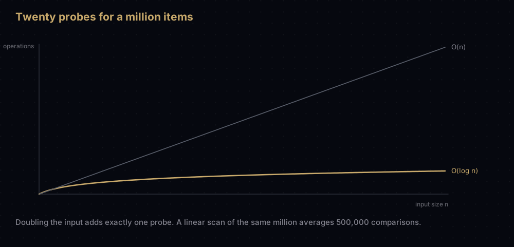
Time: O(log n). Here is the counting argument. Let the window hold m items. One probe removes the middle item and one of the two sides, leaving at most ceil((m - 1) / 2) items, which is never more than m / 2. So the window sizes are bounded by n, n/2, n/4, n/8, and so on. The search stops when the size reaches 0, and the number of halvings needed to take n down to nothing is floor(log2(n)) + 1.
That formula is exact, not a hand wave. Ten items: floor(3.32) + 1 = 4 probes, which is exactly what the failed search for 40 cost. A hundred items walk 100, 50, 25, 12, 6, 3, 1, 0: seven probes, and floor(log2(100)) + 1 = 7.
| Items | Worst-case probes | Linear scan, average |
|---|---|---|
| 10 | 4 | 5 |
| 100 | 7 | 50 |
| 1,000 | 10 | 500 |
| 1,000,000 | 20 | 500,000 |
| 1,000,000,000 | 30 | 500,000,000 |
The interesting column is the middle one, because of how slowly it moves. Doubling the data adds exactly one probe: log2(2n) = log2(n) + 1. Going from a thousand items to a billion — a million times more data — costs twenty extra comparisons.
Best case: O(1). The first probe lands on the target.
Space: O(1) for the iterative version. It keeps three integers no matter how big the list is, and it never copies anything — note that the traced version above slices items[low:high + 1] purely to print, which is O(n) work the real function does not do. The recursive version is O(log n) because each pending call holds a stack frame, and the depth is the number of probes.
Two costs are easy to forget. Getting the data sorted in the first place is O(n log n), which dwarfs any single search: linear search is the better choice if you only ever ask one question. And on very large arrays each probe jumps to an unpredictable address, so binary search misses the CPU cache on nearly every step while a linear scan streams through memory. Below a few dozen items, scanning usually wins in wall-clock time despite losing on paper.
The overflow bug that hid for nine years
Most textbooks write the middle as (low + high) // 2. In Python that is perfectly safe. Wherever the index is a fixed 32-bit int it is a latent bug: once low + high passes 2,147,483,647 the sum no longer fits. Java is the clearest case, because an array's length there is an int, so every index is one too; C and C++ code that indexes with int instead of size_t has the same hole. Java defines that overflow to wrap around to a negative number, C and C++ leave it undefined and in practice wrap the same way, and either way the division keeps the result negative and the program indexes an array with a negative subscript.
def as_int32(value: int) -> int:
    """The value a 32-bit signed integer would hold after wrapping around."""
    return (value + 2 ** 31) % 2 ** 32 - 2 ** 31


low, high = 1_500_000_000, 2_000_000_000
print("Python, (low + high) // 2:      ", (low + high) // 2)
print("32-bit, (low + high) // 2:      ", as_int32(low + high) // 2)
print("either, low + (high - low) // 2:", low + (high - low) // 2)Python, (low + high) // 2: 1750000000
32-bit, (low + high) // 2: -397483648
either, low + (high - low) // 2: 1750000000This is not a hypothetical. Joshua Bloch wrote the binary search in Java's java.util.Arrays, and in a 2006 post titled "Nearly All Binary Searches and Mergesorts are Broken" he reported that this exact overflow had been sitting in the JDK for about nine years before a real program with a large enough array finally tripped over it. The same bug was in the version Bentley published and proved correct in Programming Pearls. His fix in Java was the unsigned shift (low + high) >>> 1; the language-independent fix is low + (high - low) // 2, since high - low is at most the array length.
Python's integers are arbitrary precision — they grow into as many machine words as they need — so neither form can overflow, and (low + high) // 2 is genuinely fine here. Write the subtraction form anyway. It costs nothing, it reads no worse, and the day you port the routine to a language with fixed-width integers it is already correct.
Lower bound, upper bound, and the bisect module
"Find this value" is the least useful question binary search can answer. The more useful one is "where would this value go?", because that also tells you the first match, the last match, how many matches there are, and the nearest neighbours.
Two variants cover it. Lower bound returns the index of the first item greater than or equal to the target. Upper bound returns the index of the first item strictly greater than it. Both are written with a half-open window — high starts one past the end and the loop runs while low < high — and neither returns early on a match, because an equal value does not settle the answer. For lower bound an equal item means the answer is at or before that index; for upper bound it means the answer is after it. That is the whole difference between the two, and it is why lower_bound tests items[middle] < target while upper_bound tests items[middle] <= target: equals go left in one and right in the other.
from bisect import bisect_left, bisect_right, insort


def lower_bound(items: list[int], target: int) -> int:
    """Index of the first item >= target: the leftmost slot target could take."""
    low, high = 0, len(items)          # high is one past the end, not the last index
    while low < high:                  # strict <, and no early exit on a match
        middle = low + (high - low) // 2
        if items[middle] < target:
            low = middle + 1
        else:
            high = middle
    return low


def upper_bound(items: list[int], target: int) -> int:
    """Index of the first item > target: the rightmost slot target could take."""
    low, high = 0, len(items)
    while low < high:
        middle = low + (high - low) // 2
        if items[middle] <= target:
            low = middle + 1
        else:
            high = middle
    return low


scores = [1, 3, 3, 3, 7, 9]
print(lower_bound(scores, 3), bisect_left(scores, 3))
print(upper_bound(scores, 3), bisect_right(scores, 3))
print(upper_bound(scores, 3) - lower_bound(scores, 3), "copies of 3")
print(lower_bound(scores, 5), bisect_left(scores, 5))

timeline = [10, 20, 30]
insort(timeline, 25)
insort(timeline, 5)
print(timeline)


def index_of(items: list[int], target: int) -> int:
    """Exact-match search built on bisect_left, as the bisect docs recommend."""
    position = bisect_left(items, target)
    if position != len(items) and items[position] == target:
        return position
    raise ValueError(f"{target} is not in the list")


print(index_of(numbers, 56))
try:
    index_of(numbers, 57)
except ValueError as error:
print(error)1 1
4 4
3 copies of 3
4 4
[5, 10, 20, 25, 30]
7
57 is not in the list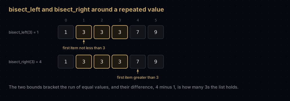
Note the high = middle lines, where the plain search wrote middle - 1. With a half-open window the item at middle has not been ruled out — it is still a candidate for the bound you are hunting — so you must not throw it away, and the window still shrinks because middle is always strictly below high while the loop is running.
In real code, do not write any of this. Python ships bisect in the standard library, implemented in C, and bisect_left and bisect_right are precisely lower_bound and upper_bound. The printed pairs above are the hand-written and library answers side by side; the last pair looks for 5, which is not in the list at all, and both report index 4: the slot where it would go. What the module gives you:
bisect_left(items, x)— index of the first item>= x. Use it for the first match, and for exact lookup via theindex_ofrecipe above, which is taken from the module's own documentation.bisect_right(items, x)— index of the first item> x. Subtract the two to count duplicates in O(log n), as the third printed line does.insort(items, x)— find the position and insert there, keeping the list sorted.- All of them take
loandhiarguments to search a slice, and since Python 3.10 akeyfunction, so you can bisect a list of records by one field.
One honest caveat about insort: the search is O(log n), but the insertion is O(n), because a Python list has to shift every later element along to make room. That shift is a fast block memory move, so a sorted list of a few thousand items with occasional inserts is completely fine, but a million-item list under constant insertion is not: reach for a heap if you only ever need the smallest item, or a balanced binary search tree if you need ordered lookups and cheap inserts at the same time.
Binary search on the answer
Here is the idea that takes binary search out of the "look up a value in a list" box, and it is the form interviews and contests actually test.
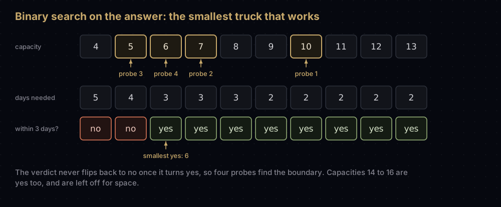
Binary search does not need a list. It needs a range of candidates and a monotonic predicate: a yes/no test that, once it starts saying yes, never goes back to no as you move up the range. That pattern looks like no, no, no, yes, yes, yes, and binary search finds the boundary between them in O(log range) tests instead of trying every candidate.
Take a concrete problem. Packages of weight [3, 2, 2, 4, 1, 4] must be loaded onto a truck in that order, one trip per day, and everything must ship within 3 days. What is the smallest truck capacity that works?
The candidate answers are capacities. Two facts bound the search: a capacity below the heaviest single package, 4, can never ship at all; a capacity equal to the total weight, 16, ships everything in one day. So the answer is somewhere in 4 to 16.
The predicate is "can this capacity finish within 3 days?", and it is monotonic for an obvious physical reason: a bigger truck never needs more days than a smaller one. So the yes-region has no holes, and the answer is the first yes.
def days_needed(weights: list[int], capacity: int) -> int:
    """Days to ship these packages, in order, with a truck of this capacity.

    Assumes capacity >= max(weights); below that no schedule exists at all.
    """
    days, load = 1, 0
    for weight in weights:
        if load + weight > capacity:   # this package starts a new day
            days += 1
            load = 0
        load += weight
    return days


packages = [3, 2, 2, 4, 1, 4]
print([days_needed(packages, capacity) for capacity in range(4, 14)])[5, 4, 3, 3, 3, 2, 2, 2, 2, 2]That list is the predicate laid bare, for capacities 4 through 13: 5 days, 4 days, then 3 or fewer from capacity 6 upwards. Never once does the day count rise as the truck grows. The answer is 6, and the point of binary search is to find it without computing that whole list.
def min_capacity(weights: list[int], deadline: int) -> int:
    """The smallest capacity that clears every package within deadline days."""
    # Below max(weights) nothing works, and sum(weights) always works in one day,
    # so the answer is somewhere in that range.
    low, high = max(weights), sum(weights)

    while low < high:
        middle = low + (high - low) // 2
        needed = days_needed(weights, middle)
        print(f"capacity {middle}: {needed} days, "
              f"{'fits' if needed <= deadline else 'too slow'}")

        if needed <= deadline:
            high = middle          # middle works, so the answer is middle or lower
        else:
            low = middle + 1       # middle fails, so the answer is above it
        print(f"  range is now {low}..{high}")

    return low


print("answer:", min_capacity(packages, 3))capacity 10: 2 days, fits
range is now 4..10
capacity 7: 3 days, fits
range is now 4..7
capacity 5: 4 days, too slow
range is now 6..7
capacity 6: 3 days, fits
range is now 6..6
answer: 6Four tests instead of thirteen. Read the shape of that loop carefully, because it is the template:
- The invariant is that everything below
lowis known to fail andhighis known to work. So the yes-branch writeshigh = middle, notmiddle - 1:middlejust proved itself a working capacity and might be the smallest one. - The no-branch writes
low = middle + 1, becausemiddleis known to fail. - The loop condition is
low < high, and it exits when the two meet on the single surviving candidate. There is noreturninside the loop and no equality test at all. You are not looking for a value, you are looking for a boundary. middlerounds down, somiddleis never equal tohighinside the loop; that is what stopshigh = middlefrom being an infinite loop.
The total cost is O(log(sum − max)) predicate tests, each costing O(n) to walk the packages. Trying every capacity would be O(n × (sum − max)). The same skeleton solves "minimum days to finish given a rate", "smallest buffer size that fits", "largest minimum distance between placed items" and the square-root-by-bisection exercise below. The hard part is never the search; it is proving the predicate is monotonic.
When to use it, and when not to
Use it when the data is already sorted and you will search it more than once. That is the whole case, and it is a common one: a sorted array of timestamps, a lookup table of thresholds, a sorted list of IDs loaded at start-up.
Use it when you need order-aware answers, not just exact hits: the nearest value, the predecessor, everything in a range, the rank of an item. A sorted array plus bisect locates any of these in O(log n) and stores the data as compactly as memory allows. Handing back a range is the one exception: finding both ends is O(log n), but copying out the k items between them is O(log n + k), and no search can beat that when you asked for k items.
Use it when the candidate answers form a monotonic range, per the section above, even when there is no list anywhere.
Do not use it for plain key lookups when a dict will do. A Python dict answers "is this key present, and what is its value" in O(1) average time, which beats O(log n), and it needs no sorting and no maintenance. Binary search wins on ordered questions, not on membership.
Do not sort just to search once. Sorting costs O(n log n); a single linear scan costs O(n) and needs no preparation.
Do not use it on a linked list. Reaching the middle costs O(n) steps, so each "halving" is linear and the whole advantage evaporates.
Do not use it on data that is not truly sorted by the same comparison you are searching with. Sorting strings by sorted() and then binary searching case-insensitively is a silent, repeatable wrong answer.
Where it shows up in the real world
Python's own standard library. random.choices builds a cumulative-weight list once and then binary searches it with bisect for every draw, turning weighted sampling into O(log n) per sample. The bisect documentation's own example maps an exam score to a letter grade by bisecting a list of breakpoints.
CPython's list.sort. Timsort binary-inserts each new element into the short run it is building, and when merging two runs it uses galloping — an exponential search followed by a binary search — to skip over long stretches from one run in one go. Every sorted() call you make runs binary searches inside.
Database indexes. A B-tree node packs many keys into one disk page, and finding which child to descend into is a binary search within that page. SQLite does exactly this on every page it visits while walking an index.
git bisect. Give it one good commit and one bad commit and it checks out the midpoint for you to test. It is binary search on the answer, with "is this commit broken" as the monotonic predicate. A thousand commits between good and bad means about ten builds, not a thousand.
Every language's standard search routine. java.util.Arrays.binarySearch, C's bsearch, Go's sort.SearchInts. C++ ships std::lower_bound and std::upper_bound: precisely the two bound functions written by hand above, and where the names used in this post come from.
Common mistakes
Searching data that is not sorted. The most common and the most dangerous, because there is no error, just a wrong answer. If the input might not be sorted, sort it once at the boundary of your code and note the precondition in the docstring.
Writing low = middle or high = middle with an inclusive window. The window stops shrinking and the process hangs, as shown above. With low <= high, the updates are always middle + 1 and middle - 1.
Mixing the two window styles. Inclusive window: high = len(items) - 1 and while low <= high. Half-open window: high = len(items) and while low < high. Pick one per function. Setting high = len(items) while keeping low <= high eventually probes index len(items) itself and raises IndexError, and it only does so when the target is larger than everything in the list: a case a quick test easily misses.
Assuming the returned index is the first match. With duplicates the plain version returns whichever equal item it happened to land on. Use bisect_left when the first one matters.
Recomputing the middle from the original bounds. middle must come from the current low and high each time round the loop, not from a value computed before the loop.
Carrying (low + high) // 2 into a fixed-width language. Safe in Python, an overflow waiting for a big enough array in Java, or in C and C++ code that indexes with int.
Forgetting that the empty result is information. When the loop ends, low is the index where the target would be inserted. Returning -1 throws that away; bisect_left hands it to you.
Practice
- Rewrite
binary_searchto return the insertion point instead of -1 when the target is missing, and check it againstbisect_lefton a list with duplicates. - Write
first_and_last(items, target)returning the first and last indices of a repeated value, using two bounded searches, and return(-1, -1)when it is absent. - Write
count_in_range(items, low_value, high_value)that counts how many items of a sorted list fall inside an inclusive range, using exactly two binary searches and no loop over the data. - Compute the integer square root of a number by binary searching the candidate answers 0 to n for the largest value whose square is at most n, and confirm it matches
math.isqrt. - Given a sorted list that has been rotated —
[38, 56, 72, 91, 2, 5, 8]— find a target in O(log n) by first binary searching for the rotation point, then searching the correct side.
Summary
Binary search is one comparison that deletes half the remaining possibilities, repeated until nothing is left. The logarithm is not a convention, it is the number of times you can halve n before reaching zero: twenty for a million, thirty for a billion. Everything that goes wrong with it goes wrong at the boundaries, so fix your window convention first (inclusive with low <= high, or half-open with low < high), and let every other line follow from it. Then use bisect and keep the hand-written version for the cases with no list in them at all.
| Difficulty | Easy |
| Best case | O(1) — the first probe lands on the target |
| Average case | O(log n) |
| Worst case | O(log n) — exactly floor(log2(n)) + 1 probes |
| Space | O(1) iterative; O(log n) recursive, for the call stack |
| Requires | Sorted data with O(1) random access |
| In place | Yes — it only reads |
| Returns first match | No — use bisect_left when that matters |
| Data structure | List / array; never a linked list |
| Use it when | The data is already sorted, or the answers form a monotonic range |
| Avoid it when | One lookup on unsorted data, or a dict would answer the question |
| Real-world use | bisect, random.choices, Timsort's galloping merge, B-tree pages, git bisect |
| Python equivalent | bisect.bisect_left(items, x) — the same algorithm, written in C |
Keep reading
- Linear Search in Python — the O(n) alternative, and the break-even maths for when sorting first actually pays.
- Big O Notation — where log n comes from and why halving is the signature of a logarithm.
- Binary Search Trees in Python — the same halving, built into a structure that also supports cheap inserts.
- Hash Tables in Python — the O(1)-average lookup that beats binary search whenever order does not matter.
- Merge Sort in Python — how the sorted input this algorithm depends on gets built, in guaranteed O(n log n).


