Linear search is the algorithm you already invented. Look at the first item. Is it the one you want? If not, look at the next one. Keep going until you find it or run out of list. There is nothing else to it.
Which makes it sound like a warm-up exercise, and mostly it is. But it is also the only search that works on data you have not prepared in any way, the only search that works on a linked list, and — for a single lookup on data nobody has sorted or indexed yet — the fastest thing available, because every cleverer alternative has to preprocess first and preprocessing costs more than the scan it saves.
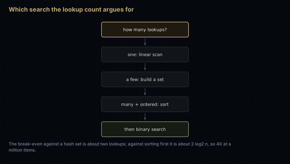
So the interesting question is never how linear search works. It is when something better actually beats it, and that has an arithmetic answer: about 2 log₂ n lookups against sorting first, and roughly two against building a hash set.
The idea
Start at index 0. Compare the item there with the target. If they match, return that index. If not, move to index 1 and repeat. Stop when you find a match or fall off the end of the list.
That is the entire mechanism, and it has one property worth naming: it assumes nothing about the data. Binary search needs the list sorted. A hash lookup needs the items hashable and a table already built. Linear search needs the list to exist, and nothing more. That is why it is the fallback that always works.
It also gives you the first match, not just a match. Because you walk left to right and return the instant you succeed, no other matching item can be at a smaller index. When a list has duplicates, that guarantee is often the whole reason you are searching.
Watching it work
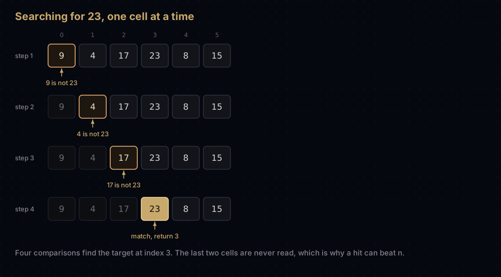
Take the list [9, 4, 17, 23, 8, 15] and search for 23.
- Index 0 holds
9. Not23. Move on. - Index 1 holds
4. Not23. Move on. - Index 2 holds
17. Not23. Move on. - Index 3 holds
23. Match — return3.
Four comparisons, and 8 and 15 were never looked at. That is the good case: the target sat near the front.
Now search the same list for 6, which is not in it.
9,4,17,23,8,15— six comparisons, six failures.- The loop runs off the end. Return
-1.
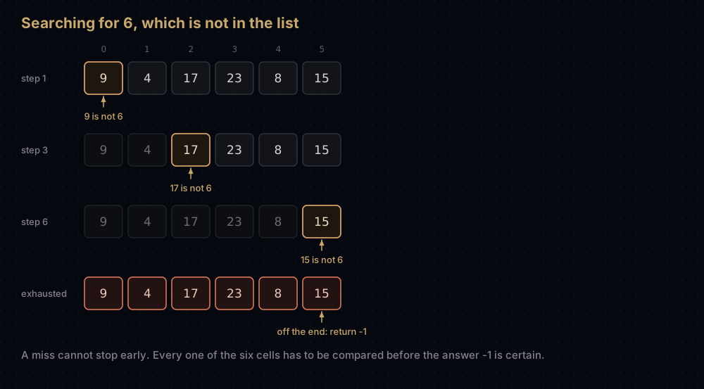
That asymmetry is the shape of the whole algorithm. A hit can stop early; a miss never can. Proving something is absent from an unsorted list means checking every single position, because the one you skipped could have been it. A failed linear search always costs exactly n comparisons. That is not an implementation weakness: with no ordering to exploit, an adversary could always put the target in the slot you chose not to read.
The code
def linear_search(values: list[int], target: int) -> int:
    """Return the index of the first item equal to target, or -1 if absent.

    Makes no assumption about order, so it works on any sequence you can
    walk from front to back.
    """
    for index in range(len(values)):
        # First match wins: nothing checked later can be at a smaller index.
        if values[index] == target:
            return index
    return -1


numbers = [9, 4, 17, 23, 8, 15]
print(linear_search(numbers, 23))
print(linear_search(numbers, 9))
print(linear_search(numbers, 6))
print(linear_search([], 6))3
0
-1
-1The empty list needs no special case: range(0) is empty, the loop never runs, and you fall through to return -1.
The sentinel trick
The loop above does two things per iteration that you might not have counted. It checks whether the index has reached the end, and it checks whether the value matches. Two tests, n times.
Sentinel search removes one of them. Plant a copy of the target in the last slot before you start. The scan is now guaranteed to stop at or before that slot, so the bounds check is dead weight and you can delete it. Afterwards, put the real value back and work out whether you stopped on a genuine match or on the sentinel.
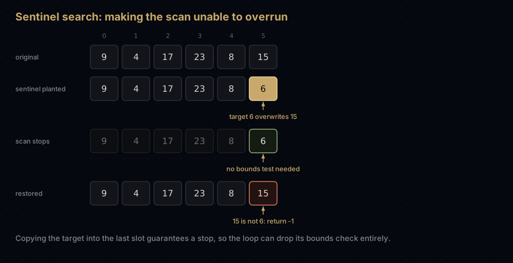
def linear_search_sentinel(values: list[int], target: int) -> int:
    """Linear search with only one test per iteration instead of two.

    Overwrites the last slot with the target so the loop is guaranteed to
    stop, which means the index bound never has to be checked. The list is
    restored before returning, but it is briefly modified, so this is not
    safe to run against a list another thread is reading.
    """
    length = len(values)
    if length == 0:
        return -1

    last_value = values[length - 1]
    values[length - 1] = target

    index = 0
    while values[index] != target:
        index += 1

    values[length - 1] = last_value

    if index < length - 1:
        return index
    # The scan stopped on the sentinel slot, so it is a real hit only if the
    # value that lived there happened to be the target.
    return length - 1 if last_value == target else -1


print(linear_search_sentinel(numbers, 23))
print(linear_search_sentinel(numbers, 15))
print(linear_search_sentinel(numbers, 6))
print(numbers)3
5
-1
[9, 4, 17, 23, 8, 15]Be honest about what this buys you. It halves the tests, not the comparisons against data, so the cost is unchanged: still O(n). In hand-written C on a hot loop it is a real win. In Python it is a loss: a while loop with manual indexing is slower than for index in range(...), and both are slower than the C-level in operator. Modern CPUs also predict the bounds branch almost perfectly, which erodes the benefit even in C.
Learn it anyway. It is the clearest small example of a technique you will meet again: make an impossible case impossible, and you get to delete the check for it.
How the code maps to the idea
The loop is the scan. range(len(values)) produces 0, 1, 2, … in order, which is exactly "start at the front and move right". Nothing in the function depends on the values being ordered, comparable, or numeric: only on == working.
The early return is the "stop when you find it". Returning from inside the loop is not tidiness; it is the reason a successful search can beat n comparisons. Replace it with a variable you assign and return at the end, and you have quietly made every search cost the full n.
The -1 is a design choice. It is the convention Java, JavaScript and most textbooks use, so you will read it constantly, but -1 is a valid Python index, so values[result] on a miss silently reads the last element instead of failing. Returning None is safer, because values[None] raises immediately. Raising ValueError, as list.index does, is right when "not found" is genuinely an error rather than an expected outcome.
Equality, not identity. The comparison is ==, so the function finds anything that compares equal to the target, not only the object you passed. For custom classes that depends entirely on how you wrote __eq__, and for floats it means 0.1 + 0.2 will not be found by searching for 0.3.
Complexity
Count the comparisons directly rather than trusting the letters:
def linear_search_counted(values: list[int], target: int) -> tuple[int, int]:
    """Same search, but also reports how many comparisons it made."""
    comparisons = 0
    for index, value in enumerate(values):
        comparisons += 1
        if value == target:
            return index, comparisons
    return -1, comparisons


for wanted in (9, 23, 15, 6):
    found_at, comparisons = linear_search_counted(numbers, wanted)
print(f"target {wanted:>2} | index {found_at:>2} | comparisons {comparisons}")target 9 | index 0 | comparisons 1
target 23 | index 3 | comparisons 4
target 15 | index 5 | comparisons 6
target 6 | index -1 | comparisons 6Best case: O(1). The target is at index 0 and the first comparison succeeds. One comparison, regardless of whether the list holds six items or six million.
Worst case: O(n). The target is at the last index, or absent. Either way every one of the n items is compared exactly once, so the count is exactly n. No constant hidden, no logarithm — n.
Average case: O(n). Suppose the target is present and equally likely to be at any of the n positions. Finding it at index i costs i + 1 comparisons, so the mean is the average of 1, 2, …, n. That sum is n(n + 1) / 2, and dividing by n gives (n + 1) / 2, about half the list. Big O drops the ½, so it is still O(n).
def average_comparisons(values: list[int]) -> float:
    """Mean comparisons when every item in the list is searched for once."""
    total = sum(linear_search_counted(values, value)[1] for value in values)
    return total / len(values)


for size in (10, 100, 1000):
    distinct = list(range(size))
    print(f"n = {size:>4} | measured {average_comparisons(distinct):>6.1f} "
f"| (n + 1) / 2 = {(size + 1) / 2:>6.1f}")n = 10 | measured 5.5 | (n + 1) / 2 = 5.5
n = 100 | measured 50.5 | (n + 1) / 2 = 50.5
n = 1000 | measured 500.5 | (n + 1) / 2 = 500.5The formula is exact, not an approximation, and the measurement matches it to the decimal.
Space: O(1). One index, one target reference, nothing that grows with the input. The sentinel variant is O(1) too. That is exactly why it overwrites the last slot rather than appending to a longer list.
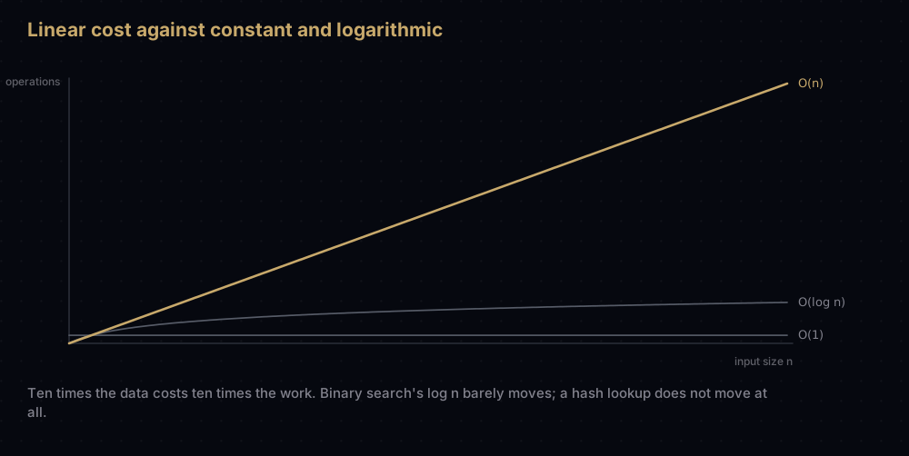
Linear growth is the mildest thing that can fairly be called slow. Ten times the data costs ten times the work: no worse, but no better either.
The break-even against sorting first
The obvious improvement is: sort the list once, then use binary search, which costs about log₂ n comparisons per lookup instead of n / 2. For a million items that is 20 comparisons instead of 500,000, a factor of 25,000.
That comparison is dishonest as stated, because it ignores the sort. Do the whole sum instead. For n items and q lookups:
- Linear search:
q * n / 2comparisons, on average, and no setup. - Sort then binary search: about
n * log2(n)comparisons once for a comparison sort, plusq * log2(n)for the lookups.
Set them equal and solve for q. The sort cost is paid once, so the question is how many lookups it takes to amortise it:
from math import ceil, log2


def break_even_lookups(n: int) -> int:
    """Lookups needed before sorting once and binary searching pays off.

    Linear search averages n / 2 comparisons per lookup. A comparison sort
    costs about n * log2(n) comparisons once, and each binary search after
    that costs about log2(n).
    """
    linear_per_lookup = n / 2
    sort_once = n * log2(n)
    binary_per_lookup = log2(n)
    return ceil(sort_once / (linear_per_lookup - binary_per_lookup))


for n in (100, 1_000, 10_000, 1_000_000):
    print(f"n = {n:>9,} | sort then binary search wins after "
f"{break_even_lookups(n):>3} lookups | 2 * log2(n) = {2 * log2(n):>4.1f}")n = 100 | sort then binary search wins after 16 lookups | 2 * log2(n) = 13.3
n = 1,000 | sort then binary search wins after 21 lookups | 2 * log2(n) = 19.9
n = 10,000 | sort then binary search wins after 27 lookups | 2 * log2(n) = 26.6
n = 1,000,000 | sort then binary search wins after 40 lookups | 2 * log2(n) = 39.9Two things fall out of that table, and both matter more than the raw numbers.
The break-even barely depends on n. Drop the small log2(n) term from the denominator and the expression collapses to n * log2(n) / (n / 2), which is just 2 log₂ n, the last column. It is loose at small n, where the exact answer is 16 rather than 13, and dead on by a million. Either way, growing the data ten-thousand-fold roughly triples the break-even. It never becomes a large number.
One lookup means linear search, always. At q = 1 you would pay 19.9 million comparisons to sort a million items in order to save 499,980. Sorting to answer a single question is about the most wasteful thing you can do with a computer, and people do it routinely because "binary search is faster" got remembered without the setup cost attached.
Against a hash set the arithmetic is even more lopsided. Building a set from n items costs about n hash operations, and each test after that is O(1) on average, so the break-even is q * n / 2 = n + q, roughly q = 2. Hashing costs more per operation than comparing, so call it a handful in practice. The conclusion stands: search the same collection more than a couple of times and you should stop searching it and build a set or a dict.
When to use it, and when not to
Use it when the data is unsorted and you are looking once. This is the common case in ordinary code: you have a list, you want one thing out of it, you move on. Anything else is premature.
Use it when the data is tiny. Under a few dozen items a linear scan usually beats binary search in wall-clock time even on sorted data: it reads consecutive memory in cache-line order and its branch pattern is trivially predictable, while binary search jumps around and mispredicts on nearly every step. At n = 20 the hardware overrules the asymptotics.
Use it when the structure gives you no choice. A singly linked list has no random access. You cannot jump to the middle without walking there first, so binary search's halving step costs O(n) and the idea collapses. The same goes for a generator, a file read line by line, or a network stream.
Use it when you are searching by a condition, not a value. "The first record whose status is failed" is not something a sorted index or a hash table can answer unless you built it on that exact field. A scan with a predicate answers it immediately.
Do not use it inside a loop over another collection. That is the accidental quadratic below, and the most common way linear search causes a real production incident.
Do not use it on a large sorted list. The bisect module already gives you binary search: bisect.bisect_left(values, target) finds the insertion point in O(log n), and you check whether the item there equals the target.
Do not use it for repeated membership testing. Build a set. Two lookups is the break-even, and the code is shorter.
Where it shows up in the real world
Unlike bubble sort, linear search is not a museum piece. You run it dozens of times a day without writing it.
Python's in operator on a list, tuple, or collections.deque is a linear scan implemented in C. So are list.index, list.count and list.remove. (Substring search is the exception: for a multi-character needle, str.find and str.count use an algorithm that can skip ahead rather than testing every position.) When you write if name in allowed_names against a list, you are running the algorithm in this post.
min, max, sum, any and all are single linear passes. any and all even short-circuit the way a search does: any stops at the first true, all at the first false.
Java's String.indexOf is a straightforward scan-and-compare rather than a clever string-matching algorithm. For the short strings most code searches, the setup cost of something like KMP would not pay for itself: the same break-even logic as above.
Hash tables finish with a linear scan. Hashing jumps you straight to a small group of candidate slots, and then keys are compared one at a time until one matches or the group runs out. The O(1) average of a hash table is really "O(1) to find a very short list, then linear search it".
Any for loop with a break is linear search wearing different clothes, which is the honest summary of why it matters. It is less an algorithm you choose than the one you fall into whenever there is no extra structure to exploit.
Python's own idioms cover most of what you would hand-write:
trees = ["ash", "birch", "cedar", "birch", "elm"]

print("birch" in trees)
print(trees.index("birch"))
print(next((i for i, name in enumerate(trees) if name.startswith("c")), -1))
print(next((i for i, name in enumerate(trees) if name.startswith("z")), -1))

try:
    trees.index("oak")
except ValueError as error:
print(f"index() raises ValueError: {error}")True
1
2
-1
index() raises ValueError: 'oak' is not in listThe next form is the one to remember. A generator expression is lazy, so next stops at the first match instead of building a full list of them — a real linear search with an early exit — and its second argument is the default on a miss, which saves you a try block.
Common mistakes
Membership testing against a list inside a loop. The classic accidental quadratic. Each in is a fresh O(n) scan, so wrapping it in a loop over m items costs O(n × m). The fix is one line.
def count_shared_slow(left: list[int], right: list[int]) -> int:
    """Quadratic by accident: every `in` restarts a full scan of `right`."""
    return sum(1 for value in left if value in right)


def count_shared_fast(left: list[int], right: list[int]) -> int:
    """Pay O(n) once to build a set, then each test is O(1) on average."""
    lookup = set(right)
    return sum(1 for value in left if value in lookup)


evens = list(range(0, 2000, 2))
thirds = list(range(0, 2000, 3))
print(count_shared_slow(evens, thirds), count_shared_fast(evens, thirds))334 334Same answer. The slow version performs up to 667,000 comparisons; the fast version performs about 1,667 hash operations: 667 to build the set, 1,000 to query it. Multiply both inputs by ten and the slow version's work grows a hundredfold while the fast version's grows tenfold, because one is quadratic and the other is linear.
Treating -1 as falsy. Writing if linear_search(values, target): looks like a not-found check and is wrong twice over: -1 is truthy, so misses pass, and 0 is falsy, so a match at index 0 fails. Compare explicitly with != -1, or return None and test with is not None.
Returning the value instead of the index. Such a function cannot distinguish "absent" from "present but equal to the sentinel you chose". Return the index.
Mutating the list while scanning it. Deleting items during a for loop over the same list shifts everything after the deletion left by one, so the loop skips the next element. Iterate over a copy.
Assuming the last match. linear_search returns the first match. If you need the last, scan reversed(range(len(values))): do not scan forwards overwriting a variable, which costs the full n every time.
Expecting in to mean ==. CPython's in checks identity before equality, which changes the answer for NaN, the one value that is not equal to itself:
not_a_number = float("nan")
print(not_a_number == not_a_number)
print(not_a_number in [not_a_number])
print(float("nan") in [float("nan")])False
True
FalseIn the middle case the list holds an object that is the target, so the identity check short-circuits before equality is consulted. Two separately constructed NaN values are different objects, so the third line falls through to == and reports False.
Practice
- Rewrite
linear_searchto returnNoneinstead of-1, and update a caller to handle it. - Write
find_allthat returns a list of every index where the target appears, and confirm it always costs exactly n comparisons. - Add a
keyparameter so you can search a list of(name, score)tuples by score alone, without unpacking at every call site. - Write
linear_search_lastthat returns the final match, and explain why scanning backwards beats scanning forwards and remembering. - Measure the crossover: time
target in a_listagainsttarget in a_setat sizes 10, 100 and 10,000, counting the cost of building the set, and find where the set starts winning.
Summary
Linear search is O(n) and cannot be improved without changing the data. That sounds like a limitation and is really its defining strength: it is the only search that asks nothing of the input. Every faster method buys its speed with preprocessing (sorting, hashing, indexing), and preprocessing has to be paid for. Do the sum before assuming the faster algorithm is faster.
| Difficulty | Easy |
| Best case | O(1) — the target is the first item |
| Average case | O(n) — exactly (n + 1) / 2 comparisons when the target is present |
| Worst case | O(n) — the target is last, or absent; every item is compared |
| Space | O(1) — one index, no extra storage |
| Data structure | Any sequence you can walk forwards: list, tuple, linked list, generator, file |
| Requires sorted input | No — this is the whole point |
| Finds | The first match, in index order |
| Use it when | The data is unsorted, tiny, or you are looking exactly once |
| Avoid it when | You will search the same collection repeatedly — build a set after about two lookups |
| Real-world use | Python's in, list.index, min, max, any; linked-list traversal; the final step of every hash-bucket lookup |
| Python equivalent | target in items / items.index(target) / next((i for i, v in enumerate(items) if v == target), -1) |
Learn the break-even arithmetic more than the algorithm. "Sort it and binary search" is right about 40 lookups into a million-item list and wrong before that, and knowing which side of the line you are on is worth more than any single search routine.
Keep reading
- Binary Search in Python — the O(log n) alternative, what it demands of your data, and how the halving argument works.
- Hash Tables in Python — how a
setturns repeated lookups into O(1), and why the last step is still a small linear scan. - Big O Notation — the full counting method behind every bound used above.
- Arrays and Dynamic Arrays — why scanning a Python list is cache-friendly, and what indexing really costs.
- Linked Lists in Python — the structure where linear search is not a choice but the only option.


