A Python list keeps values in order by keeping them in position: index 0, then 1, then 2. That is what makes binary search fast. You jump to the middle in one step. It is also what makes inserting into the middle of a sorted list cost O(n), because every value after the insertion point shifts one slot right.
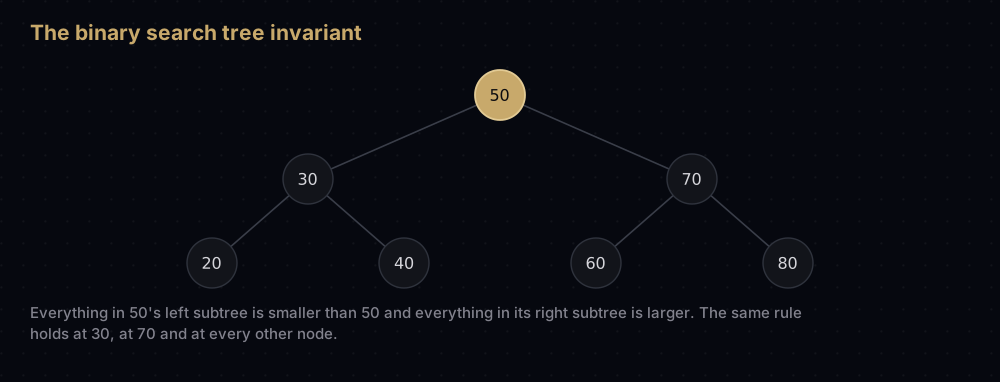
A binary search tree stores the same ordering in links instead of positions. Each node holds one value and points at up to two children, and one rule holds at every node: every value in the left subtree is smaller than the node, and every value in the right subtree is larger. Nothing moves when you insert. You follow the rule down to an empty slot and hang a new node there.
That one rule gives you search, insert, delete, minimum, maximum and sorted output from a single structure. It also comes with a catch this post will not hide: every search, insert and delete costs the height of the tree, and a plain binary search tree does nothing to keep the height small. Feed it sorted values and it degrades into a linked list.
The idea
A binary search tree — BST from here on — is made of nodes. Each node stores a value and links to a left and a right child; either link may be empty. The top node is the root, a node with no children is a leaf, and the tree grows downwards.
The rule that makes it a search tree, usually called the BST invariant, is this:
For every node, every value in its left subtree is smaller than the node's value, and every value in its right subtree is larger.
The word subtree is doing the work there. It is not enough for the left child to be smaller: every value anywhere down the left branch must be smaller, however deep. That stronger version is what makes search work.
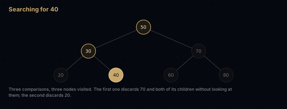
Here is why that pays off. You are looking for 40, standing at the root, which holds 50. One comparison: 40 is smaller, so the invariant guarantees 40 cannot be in the right subtree, not the right child, not anything below it. An entire subtree is eliminated without a single node in it being read. Repeat at the left child and another subtree goes.
Search never backtracks and never branches. It walks one path from the root downwards, ending when it finds the value or falls off the bottom into an empty slot. So a search costs the length of that path, and the longest path in the tree is its height, h. Search, insert and delete are all O(h), and everything interesting about a BST comes down to what h turns out to be.
Watching it work
Insert these seven values, left to right: 50, 30, 70, 20, 40, 60, 80. Insertion runs the same walk as search (compare, turn, repeat), and puts the new node in the first empty slot it reaches.
- 50 — the tree is empty, so 50 becomes the root.
- 30 — smaller than 50, turn left. That slot is empty: 30 becomes 50's left child.
- 70 — larger than 50, turn right. Empty: 70 becomes 50's right child.
- 20 — smaller than 50, left to 30. Smaller than 30, left again. Empty: 20 is 30's left child.
- 40 — smaller than 50, left to 30. Larger than 30, right. Empty: 40 is 30's right child.
- 60 — larger than 50, right to 70. Smaller than 70, left. Empty: 60 is 70's left child.
- 80 — larger than 50, right to 70. Larger than 70, right. Empty: 80 is 70's right child.
The tree that comes out looks like this:
               50
             /   \
         30          70
       /   \       /   \
      20    40    60    80
The deepest nodes sit two edges below the root, so h is 2 and no search ever reads more than 3 of the 7 values. Search for 40, starting at the root:
- 40 against 50 — smaller, go left. Nodes 70, 60 and 80 are permanently out of the running.
- 40 against 30 — larger, go right. Node 20 is out.
- 40 against 40 — found, after three comparisons.
A failed search stops the same way. Looking for 65: larger than 50, go right to 70; smaller than 70, go left to 60; larger than 60, go right, and that slot is empty. The empty slot is the answer, and it is also exactly where 65 would go if you inserted it. Insert and search are the same walk.
The code
Nodes, insert and search
A node is a small class. Insert and search are loops rather than recursion here, because both walk a single path and a loop makes that obvious.
class Node:
    """One node of a binary search tree: a value plus up to two children."""

    def __init__(self, value: int) -> None:
        self.value = value
        self.left: "Node | None" = None
        self.right: "Node | None" = None


def insert(root: "Node | None", value: int) -> Node:
    """Insert a value and return the root of the tree it belongs to.

    Walks down from the root taking one turn per node, then hangs the new
    node off the empty slot it lands in. Duplicates are ignored, so the tree
    stores a set of values.
    """
    if root is None:
        return Node(value)

    current = root
    while True:
        if value < current.value:
            if current.left is None:
                current.left = Node(value)
                return root
            current = current.left
        elif value > current.value:
            if current.right is None:
                current.right = Node(value)
                return root
            current = current.right
        else:
            return root


def search(root: "Node | None", value: int) -> bool:
    """True if the value is in the tree."""
    current = root
    while current is not None:
        if value == current.value:
            return True
        # One comparison, one turn: the other subtree is discarded untouched.
        current = current.left if value < current.value else current.right
    return False


def search_path(root: "Node | None", value: int) -> list:
    """The values a search visits, in order, whether or not it finds the target."""
    path, current = [], root
    while current is not None:
        path.append(current.value)
        if value == current.value:
            break
        current = current.left if value < current.value else current.right
    return path


root = None
for value in [50, 30, 70, 20, 40, 60, 80]:
    root = insert(root, value)

print("contains 40:", search(root, 40))
print("contains 65:", search(root, 65))
print("path to 40: ", search_path(root, 40))
print("path to 65: ", search_path(root, 65))contains 40: True
contains 65: False
path to 40: [50, 30, 40]
path to 65: [50, 70, 60]Those two paths are the walkthrough above, printed by the real code.
The four traversals
A traversal visits every node exactly once. There are four worth knowing: three walk down the tree and differ only in when a node is handled relative to its children, and the fourth walks across it a row at a time.
def in_order(node: "Node | None", out: list) -> list:
    """Left subtree, node, right subtree — visits values in ascending order."""
    if node is None:
        return out
    in_order(node.left, out)
    out.append(node.value)
    in_order(node.right, out)
    return out


def pre_order(node: "Node | None", out: list) -> list:
    """Node before its children — the order that rebuilds this exact tree."""
    if node is None:
        return out
    out.append(node.value)
    pre_order(node.left, out)
    pre_order(node.right, out)
    return out


def post_order(node: "Node | None", out: list) -> list:
    """Both children before the node — the order that is safe to free in."""
    if node is None:
        return out
    post_order(node.left, out)
    post_order(node.right, out)
    out.append(node.value)
    return out


from collections import deque


def level_order(root: "Node | None") -> list:
    """Row by row, left to right — breadth-first search over the tree."""
    if root is None:
        return []
    order, queue = [], deque([root])
    while queue:
        node = queue.popleft()
        order.append(node.value)
        if node.left is not None:
            queue.append(node.left)
        if node.right is not None:
            queue.append(node.right)
    return order


print("in-order:   ", in_order(root, []))
print("pre-order:  ", pre_order(root, []))
print("post-order: ", post_order(root, []))
print("level-order:", level_order(root))in-order: [20, 30, 40, 50, 60, 70, 80]
pre-order: [50, 30, 20, 40, 70, 60, 80]
post-order: [20, 40, 30, 60, 80, 70, 50]
level-order: [50, 30, 70, 20, 40, 60, 80]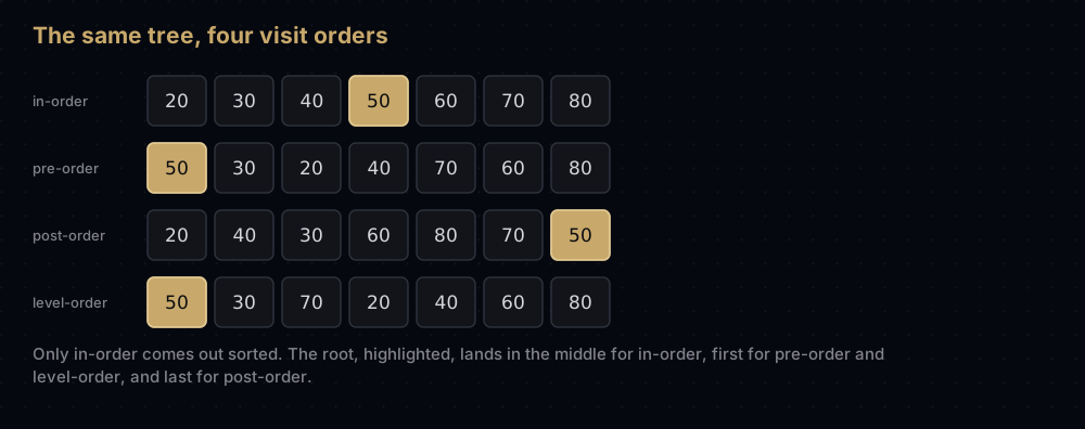
In-order comes out sorted, and that is not a coincidence. At any node, everything in the left subtree is smaller and everything in the right subtree is larger. In-order emits the whole left subtree, then the node, then the whole right subtree, so every smaller value appears before the node and every larger one after it. Apply the same argument inside each subtree and the entire output is ascending. Sorting a BST is one O(n) walk, because the insertions already did the sorting.
Pre-order emits a node before its children, so each subtree's root arrives before anything that belongs under it. Re-inserting a pre-order sequence into an empty tree therefore rebuilds the identical tree, which makes it the order to serialise in.
Post-order handles a node only once everything below it is finished. That is the order you free a tree in, and the order you evaluate an expression tree in. You need both operands before you can apply the operator.
Level-order goes row by row using a queue, which is breadth-first search applied to a tree. The other three are depth-first and cost O(h) stack; level-order's queue can hold a whole level, about n/2 nodes at the bottom of a full tree, so O(n) memory.
Delete, and its three cases
Deletion is the only fiddly operation, because removing a node leaves a hole that has to be filled without breaking the invariant. There are three cases.
- A leaf. No children, no hole to fill. Detach it.
- One child. That child's subtree slots straight into the gap. Everything in it already sits on the correct side of the deleted node's parent, so the invariant survives.
- Two children. Neither child can be promoted, because each brings a whole subtree and there is only one slot. Find instead a value that is allowed to sit there: the in-order successor, the smallest value in the right subtree. Copy it into the node, then delete the successor from the right subtree. It is the leftmost node, so it has no left child, which means that second delete is case 1 or case 2.
def find_min(node: Node) -> Node:
    """The leftmost node of a subtree, which holds its smallest value."""
    while node.left is not None:
        node = node.left
    return node


def delete(node: "Node | None", value: int) -> "Node | None":
    """Delete a value from the subtree at node, returning the new subtree root.

    The caller reattaches the returned node, which is what makes all three
    cases work with one line each.
    """
    if node is None:
        return None

    if value < node.value:
        node.left = delete(node.left, value)
    elif value > node.value:
        node.right = delete(node.right, value)
    else:
        # Cases 1 and 2 collapse into one: promote whichever child exists.
        # A leaf has no children, so this returns None and the node vanishes.
        if node.left is None:
            return node.right
        if node.right is None:
            return node.left

        # Case 3: two children. The in-order successor is the smallest value
        # in the right subtree, so it is larger than everything on the left
        # and smaller than everything else on the right — exactly what this
        # slot requires.
        successor = find_min(node.right)
        node.value = successor.value
        node.right = delete(node.right, successor.value)

    return node


tree = None
for value in [50, 30, 70, 20, 40, 60, 80]:
    tree = insert(tree, value)

tree = delete(tree, 20)
print("deleted 20 (leaf):        ", in_order(tree, []))
tree = delete(tree, 30)
print("deleted 30 (one child):   ", in_order(tree, []))
tree = delete(tree, 50)
print("deleted 50 (two children):", in_order(tree, []))
print("root is now:              ", tree.value)
print("still a valid BST: ", in_order(tree, []) == sorted(in_order(tree, [])))deleted 20 (leaf): [30, 40, 50, 60, 70, 80]
deleted 30 (one child): [40, 50, 60, 70, 80]
deleted 50 (two children): [40, 60, 70, 80]
root is now: 60
still a valid BST: TrueThe third case deserves a hand-trace, because it is the one people get wrong. Take the original seven-node tree and delete 50, the root. Go right once to 70, then left as far as possible: that lands on 60, the smallest value in the right subtree. Copy 60 into the root, then delete 60 from the right subtree. It is a leaf, so it detaches, and 70 is left holding only its right child, 80.
The run above reaches the same successor from a smaller tree, because by the time it deletes 50 the right subtree is still untouched.
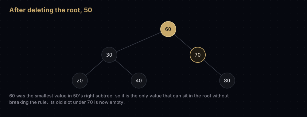
The in-order predecessor — the largest value in the left subtree — works just as well, for the mirror-image reason. Always choosing the successor makes the tree lean left over many deletions, which is one more argument for balancing.
How the code maps to the idea
insert and search are the same walk. Both compare, turn and repeat, and neither ever backtracks. The only difference is what happens at an empty slot: search returns False, insert puts a node there.
Duplicates are dropped. The final else in insert — the value equals the current node — returns without doing anything, so this tree behaves like a set. The alternative is a count on each node. What you must not do is send equal values down an arbitrary side, or search can walk past a match and never see it.
delete returns the new subtree root and the caller reassigns. node.left = delete(node.left, value) looks like busywork, but it is what makes deletion work with no parent pointers. Whatever the recursive call decides (an unchanged node, a promoted child, or None) the parent stores the result in the slot it came from. Deleting the root is the same move one level up: tree = delete(tree, value).
The three delete cases are really two. A leaf has no left child, so if node.left is None: return node.right returns None and the node disappears; a node with only a right child hits that same line and returns the child. Case 1 is case 2 with an empty subtree, which is why there is no leaf-specific branch.
find_min walks left. The smallest value in a subtree is its leftmost node: anything smaller would have to be in a left subtree, so keep going left until there is none.
Edge cases all fall out of the two None guards. insert(None, v) returns a fresh root, so an empty tree needs no special case. delete(None, v), and deleting a value that is not there, both hit if node is None: return None and quietly do nothing. Deleting the only node of a one-node tree returns None, leaving an empty tree.
Complexity
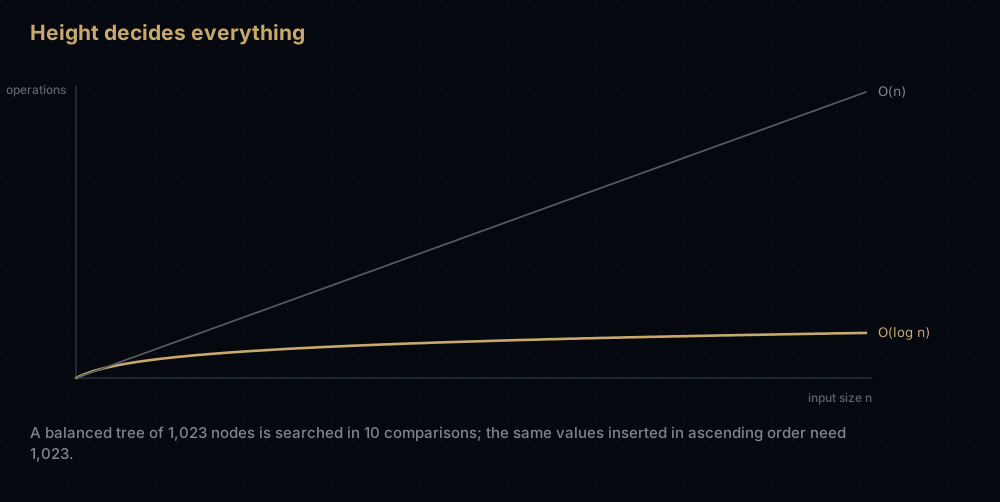
Every single-value operation (search, insert, delete, minimum, maximum) walks one root-to-leaf path and does O(1) work per node. So they are all O(h), where h is the height of the tree measured in edges. The whole analysis is therefore a question about h.
The best possible height. A tree of height h holds 1 node on its first level, at most 2 on the second, at most 4 on the third, and so on, so at most 2^(h+1) - 1 nodes altogether. Turn that around and a tree of n nodes needs h of at least log2(n + 1) - 1, a bound a perfectly balanced tree hits exactly. For 1,023 nodes the height is 9 edges, so a search reads 10 values out of 1,023: the halving argument from binary search, rebuilt out of pointers.
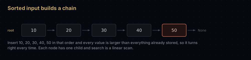
The worst possible height. If every value inserted is larger than everything already stored, every insert turns right and the tree is a single chain of n nodes with h = n - 1. Search becomes a linear scan of a memory-hungry linked list.
The average depth. Averaged over all n! insertion orders, the expected depth of a node is about 1.39 * log2 n, roughly 39% worse than perfect, and that depth is what a search pays. The expected height is higher, about 2.99 * log2 n, but still logarithmic. That is why a BST copes with shuffled data. It is not a guarantee, because real data is very often nearly sorted: timestamps, auto-increment IDs, alphabetised names.
Building a tree of n values costs the sum of the individual inserts. Balanced, that is n inserts at O(log n) each, so O(n log n). In sorted order, the i-th insert walks past all i - 1 existing nodes, giving 1 + 2 + ... + (n - 1) = n(n - 1) / 2 comparisons: O(n²) just to build.
Here is that degradation with real numbers rather than a promise:
def balanced_order(values: list) -> list:
    """Reorder a sorted list so inserting it left to right builds a balanced tree."""
    if not values:
        return []
    middle = len(values) // 2
    return ([values[middle]]
            + balanced_order(values[:middle])
            + balanced_order(values[middle + 1:]))


ascending = list(range(1, 1024))

degenerate = None
for value in ascending:
    degenerate = insert(degenerate, value)

balanced = None
for value in balanced_order(ascending):
    balanced = insert(balanced, value)

print("1023 values, searching for the largest one")
print("  sorted insert order:  ", len(search_path(degenerate, 1023)), "nodes visited")
print("  balanced insert order:", len(search_path(balanced, 1023)), "nodes visited")

for label, subject in [("sorted  ", degenerate), ("balanced", balanced)]:
    try:
        print(f"  recursive in-order, {label} tree: {len(in_order(subject, []))} values")
    except RecursionError:
print(f" recursive in-order, {label} tree: RecursionError")1023 values, searching for the largest one
sorted insert order: 1023 nodes visited
balanced insert order: 10 nodes visited
recursive in-order, sorted tree: RecursionError
recursive in-order, balanced tree: 1023 valuesSame 1,023 values, same code, same invariant, and a hundredfold difference in search cost decided entirely by arrival order. The last two lines show the second failure mode: the sorted-order tree is 1,023 nodes deep, which blows CPython's default recursion limit of 1,000 before the traversal finishes. Imbalance does not only make a tree slow, it makes ordinary recursive code crash.
| Nodes | Balanced path length | Sorted-insert path length |
|---|---|---|
| 15 | 4 | 15 |
| 1,023 | 10 | 1,023 |
| 1,048,575 | 20 | 1,048,575 |
Traversals are O(n) — every node is visited exactly once and does constant work. A range query is O(h + k), not O(h): one walk down to the low end, then one step per value emitted, so the k matches dominate once the range is wide. Space is O(n) for the nodes, each an object holding a value and two references, plus O(h) for the call stack during a recursive traversal or a recursive delete.
When to use it, and when not to
Use an ordered tree when you need order plus mutation. The queries a hash table cannot answer at all are the ones a BST is built for: minimum and maximum, "the smallest key greater than x", every record between two timestamps, and iteration in sorted order — all while inserts and deletes keep arriving. A sorted list answers those queries but pays O(n) per insert; a BST keeps insert, delete, minimum, maximum and successor at O(h), and a range query at O(h + k).
Do not use a plain, unbalanced BST in production. Nothing in this post's code stops the tree degenerating, and the inputs that degenerate it are the common ones. The fix is a tree that rebalances itself as it changes, which costs a rotation or two per insert and buys a hard O(log n) guarantee. That is AVL trees and their relatives, the natural next post.
If you only need lookup by key, use a dict. Hash tables give O(1) average lookup and nothing here beats it. The trade is that a dict has no order: it cannot answer "what is the next key after this one" without scanning everything.
If the data is static, sort it once and use bisect. bisect_left does binary search over a sorted list in O(log n) with none of the pointer overhead. And if you only ever need the smallest item, heapq maintains the minimum in O(log n) without keeping the rest sorted at all. That is heaps and priority queues.
Where it shows up in the real world
Database indexes are the biggest deployment of this idea. SQLite, PostgreSQL and MySQL's InnoDB engine build their default indexes as B-trees or B+ trees, which generalise the BST rule to many keys and many children per node so one node fills a disk page. The ordering is the same one from the top of this post, and it is why WHERE created_at BETWEEN ... can use an index while WHERE lower(name) = ... often cannot.
The Linux kernel ships a red-black tree, rbtree, as a core library: a BST that rebalances on every insert and delete. epoll uses one to store the file descriptors a program is watching, and the CPU scheduler keeps its runnable tasks in one ordered by virtual runtime, which is what lets it pick the next task to run without scanning them all.
Standard libraries expose them as ordered maps. Java's TreeMap and TreeSet, and C++'s std::map and std::set, are balanced binary search trees: red-black trees in the usual implementations. That is why iterating a TreeMap gives you sorted keys and iterating a HashMap does not.
Python is the odd one out: it ships no tree-based container. dict and set are hash tables, and the standard library's answer for ordered data is bisect over a list. Even the popular third-party sortedcontainers avoids trees: it keeps a list of short lists, because in CPython, locality and C-level list operations beat one Python object per node. That is a lesson about constant factors, not a reason to skip the theory: in C, Java, Go and Rust, ordered trees are everywhere.
Common mistakes
Forgetting to reassign the result of delete. Writing delete(node.left, value) without the node.left = in front discards the new subtree root. The value looks deleted inside the recursive call and is still there afterwards. This is the single most common BST bug.
Validating the invariant by looking only at children. A check that tests node.left.value < node.value at every node accepts broken trees. Take a root of 20 with a right child of 30 that has a left child of 10: every parent-child pair looks fine, but 10 sits in 20's right subtree, so a search for 10 turns left at the root and never finds it. Validate by passing a permitted (low, high) range down the recursion, narrowing it at each step.
Promoting a child when deleting a node with two children. Attaching the left child in the gap orphans the right subtree, or forces you to re-insert it node by node. The successor or predecessor is the only value that fits without moving anything else.
Feeding the tree sorted data. Loading rows ordered by primary key or timestamp builds the chain shown above. If you must use an unbalanced BST, shuffle the input first.
Using a mutable default argument for the traversal accumulator. def in_order(node, out=[]) gives every call the same list, because defaults are evaluated once when the function is defined, so the second traversal appends to the first one's results. Pass the list explicitly, as the code above does.
Practice
- Write
find_maxas the mirror offind_minand print the smallest and largest values without traversing the whole tree. - Write
height(node), returning the number of edges on the longest downward path and -1 for an empty tree: then write it iteratively, so it survives the 1,023-node chain from the complexity section. - Write
is_valid_bst(node)by passing a permitted(low, high)range down the recursion, and test it on the broken 20 / 30 / 10 tree from Common mistakes. - Change
deleteto use the in-order predecessor instead of the successor, and confirm the in-order output after each deletion is unchanged. - Write
values_between(node, low, high), skipping any subtree that cannot contain a match, at a node smaller thanlow, the whole left subtree can be ignored.
Summary
A binary search tree is one rule applied everywhere: smaller on the left, larger on the right, all the way down. That rule turns search into a single walk from the root, hands you sorted output from an in-order traversal, and keeps minimum, maximum and range queries cheap while the data keeps changing. Every search, insert and delete costs the height of the tree, and that is the catch. Height is only log2 n while the tree stays balanced, and nothing here enforces balance: 1,023 values inserted in ascending order cost 1,023 comparisons per search instead of 10. Learn the invariant and the traversals here, then reach for a self-balancing version before shipping anything.
| Difficulty | Medium |
| Best case | O(log n) — balanced tree, one root-to-leaf walk |
| Average case | O(log n) — random insertion order, about 1.39 times the perfect depth |
| Worst case | O(n) — sorted input builds a single chain |
| Search / insert / delete | O(h), where h is the height of the tree |
| Range query | O(h + k) — the walk down, plus one step per value returned |
| Traversal | O(n) — every node visited once |
| Space | O(n) nodes, plus O(h) call stack for recursive traversal |
| Sorted output | Yes — an in-order traversal, in O(n) |
| Self-balancing | No — that is what AVL and red-black trees add |
| Data structure | Linked nodes, up to two children each |
| Use it when | You need ordered operations (min, max, ranges, successor) on data that keeps changing |
| Avoid it when | Keys arrive in sorted order, or plain key lookup is all you need |
| Real-world use | The basis of red-black trees (Linux rbtree, Java TreeMap) and B-trees (database indexes) |
| Python equivalent | None built in — bisect over a sorted list, or dict when order does not matter |
Keep reading
- AVL Trees and Self-Balancing — the rotations that keep the height at log n and fix the worst case shown here.
- Binary Search in Python — the same halving argument on a plain array, and the
bisectmodule. - Hash Tables in Python — O(1) lookups when you do not need any ordering.
- Heaps and Priority Queues — a different tree with a weaker invariant, when only the smallest item matters.
- Breadth-First Search — level-order traversal generalised from trees to graphs.


