Breadth-first search is the algorithm for "how far?" when every step costs the same. Fewest moves to solve a sliding puzzle, shortest route through a maze, how many handshakes separate you from a stranger: one problem wearing three costumes, and BFS solves it in about fifteen lines of Python.
The mechanism is almost embarrassingly simple. Keep a queue of places you have found but not yet looked at, always take the oldest one out, and put its unseen neighbours at the back. That rule makes the search spread outwards in rings of equal distance, which is why the first time BFS reaches a node it has arrived by the fewest possible edges. Swap the queue for a stack and you get depth-first search: same nodes, no shortest-path guarantee.
What follows builds BFS three times (plain traversal, traversal by level, then a shortest-path function with parent tracking) runs it on a grid maze, earns the O(V + E) bound by counting, and shows the one-line slip that turns a correct BFS into a memory hog.
The idea
A graph is a collection of things and the links between them. The things are nodes: people, cities, web pages, cells in a maze. The links are edges: a friendship, a road, a hyperlink, a legal move. Edges are undirected when they work both ways and directed when they do not. A graph is unweighted when every edge costs the same to cross: the only kind BFS handles. In Python you store one as an adjacency list, a dictionary mapping each node to the nodes it links to: {"A": ["B", "C"], "B": ["A"]} says A joins to B and C, and B joins back to A.
Start at one node, the source, and keep two things: a queue of nodes discovered but not yet examined, and a visited set of nodes already queued. Put the source in both. Then repeat until the queue is empty: take the node at the front, look at each neighbour, and for any neighbour not already in the visited set, add it to the set and push it onto the back.
Because new nodes always go on the back and you always take from the front, everything one edge from the source leaves the queue before anything two edges away. The search fans out in rings.
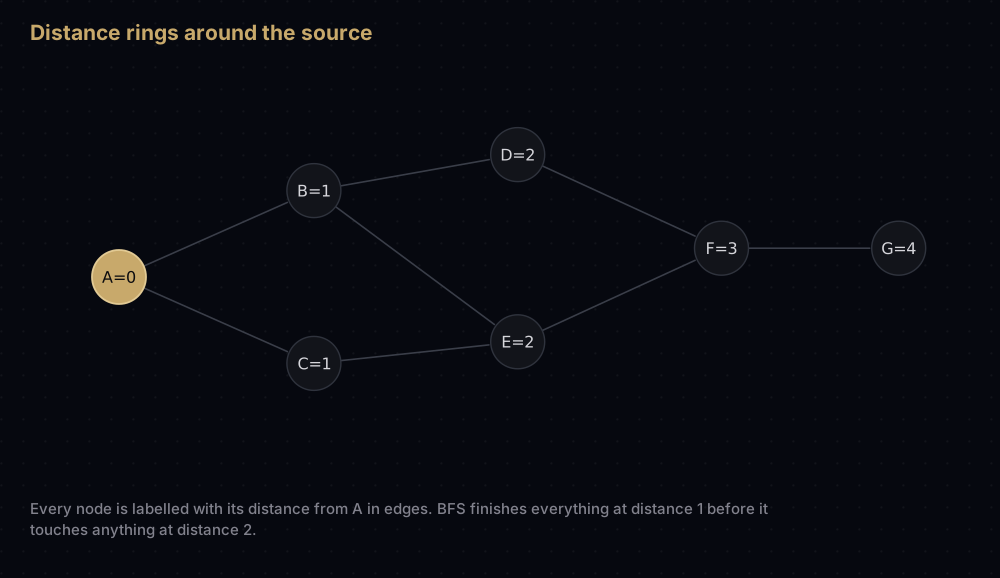
Why the first arrival is the shortest arrival
Give every node the distance it was assigned when it entered the queue: the source gets 0, and a node discovered while examining a node at distance d gets d + 1. Now look at what the queue can hold. It starts with the source alone, and every pop of a distance-d node pushes distance-d + 1 nodes onto the back, so the queue always holds a run of d followed by a run of d + 1, and nothing else. Distances leave the queue in non-decreasing order.
That gives the result. Say the true shortest route to v is k edges, and the node just before v on it is u, at distance k - 1. Since pops happen in non-decreasing distance order, nothing further away than u has popped by the time u does. So either v is still unvisited when u is examined and gets exactly k, or an earlier pop — at distance k - 1 or less — already gave it at most k. It cannot be under k either, because following the parent pointers back yields a real path of that length. So it is exactly k.
A stack breaks that argument at once. Take the newest node rather than the oldest and the search dives to the bottom of one branch before it looks at the source's second neighbour, so it can reach a node the long way first and mark it done.
Watching it work
Here is the graph from the diagram, written as an adjacency list. It is undirected, so each edge shows up in two places.
A: B, C
B: A, D, E
C: A, E
D: B, F
E: B, C, F
F: D, E, G
G: F
Start at A, with A in both the visited set and the queue.
Pop A. B and C are new: mark both, push both. Queue: B, C.
Pop B. A is visited; D and E are new. Queue: C, D, E.
Pop C. A is visited, and so is E: B marked it a moment ago, even though E has not been examined yet. Nothing is pushed. Queue: D, E. Remember this step: E already belongs to B, and C correctly leaves it alone.
Pop D. F is new. Queue: E, F. Pop E. Everything it touches is visited. Queue: F.
Pop F. G is new. Queue: G. Pop G. Its only neighbour is visited, the queue empties, and the traversal is over.
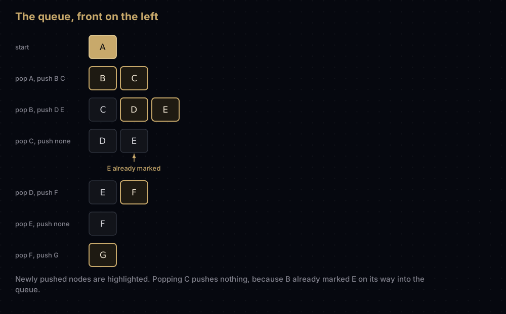
Visit order: A, B, C, D, E, F, G. Distances: A 0, B and C 1, D and E 2, F 3, G 4. Seven pops, one per node, and every edge looked at exactly twice: once from each end.
Remembering how you got there
That tells you which nodes are reachable, not how to reach them. Fixing it costs one dictionary: every time you mark a neighbour, record which node discovered it.
Here A discovered B and C, B discovered D and E, D discovered F, F discovered G. To get from A to G, start at G and follow those pointers backwards (G, F, D, B, A) then reverse. The result, A, B, D, F, G, is four edges, matching G's distance exactly. It has to: each pointer step drops the distance by one.
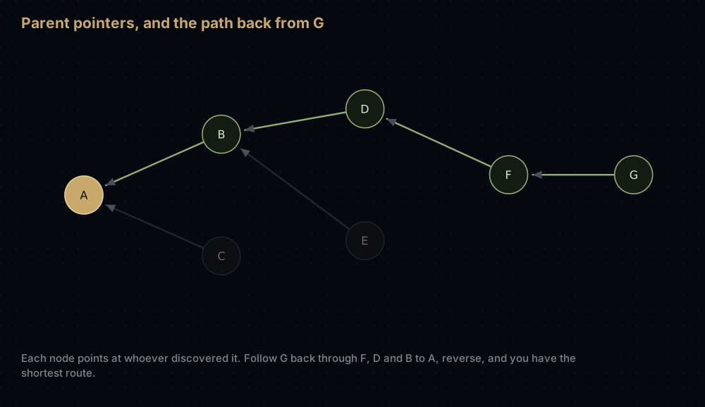
Those pointers form the BFS tree: every node but the source has exactly one parent. Note that E points at B, not C, although both are one edge from A and both border E. B got there first. When several shortest paths exist, BFS returns one of them, picked by adjacency-list order.
The code
The plain traversal first. Everything later is a variation on it.
from __future__ import annotations  # lets the hints below use "X | None" on older Pythons

from collections import deque

# An adjacency list: every key is a node, every value is the nodes it links to.
# This graph is undirected, so each edge appears in both directions.
graph: dict[str, list[str]] = {
    "A": ["B", "C"],
    "B": ["A", "D", "E"],
    "C": ["A", "E"],
    "D": ["B", "F"],
    "E": ["B", "C", "F"],
    "F": ["D", "E", "G"],
    "G": ["F"],
}


def bfs_order(graph: dict[str, list[str]], source: str) -> list[str]:
    """Return every node reachable from source, in breadth-first order."""
    visited = {source}          # marked the moment a node is queued, never later
    queue = deque([source])     # deque, because popping from the left must be O(1)
    order: list[str] = []

    while queue:
        node = queue.popleft()  # the oldest node in the queue, so the nearest one
        order.append(node)
        for neighbour in graph[node]:
            if neighbour not in visited:
                visited.add(neighbour)
                queue.append(neighbour)

    return order


print(bfs_order(graph, "A"))
print(bfs_order(graph, "G"))['A', 'B', 'C', 'D', 'E', 'F', 'G']
['G', 'F', 'D', 'E', 'B', 'C', 'A']Starting from G gives a completely different order, because the rings are now centred on G. BFS order is a property of the source, not of the graph.
Often you want the levels themselves: "everyone exactly three hops away". Drain the entire current ring before starting the next and the boundaries fall out for free.
def bfs_levels(graph: dict[str, list[str]], source: str) -> list[list[str]]:
    """Group every reachable node by its distance in edges from source."""
    visited = {source}
    frontier = [source]
    levels: list[list[str]] = []

    while frontier:
        levels.append(frontier)
        next_frontier: list[str] = []
        # Drain the whole current ring before starting the next one, which is
        # what makes the level boundaries explicit instead of implied.
        for node in frontier:
            for neighbour in graph[node]:
                if neighbour not in visited:
                    visited.add(neighbour)
                    next_frontier.append(neighbour)
        frontier = next_frontier

    return levels


for level_number, level in enumerate(bfs_levels(graph, "A")):
print(level_number, level)0 ['A']
1 ['B', 'C']
2 ['D', 'E']
3 ['F']
4 ['G']No queue at all: two lists take turns. Same work, same order, and often the clearer shape when the level number matters, since the distance is the index rather than something you store.
Now the version you will actually use: shortest path, with parent tracking and reconstruction.
from typing import TypeVar

Node = TypeVar("Node")


def reconstruct(parent: dict[Node, Node | None], target: Node) -> list[Node]:
    """Walk the parent chain back from target, then reverse it."""
    path: list[Node] = []
    node: Node | None = target
    while node is not None:
        path.append(node)
        node = parent[node]
    path.reverse()
    return path


def bfs_shortest_path(graph: dict[str, list[str]], source: str,
                      target: str) -> list[str] | None:
    """Fewest-edges path from source to target, or None if none exists."""
    if source == target:
        return [source]

    # parent doubles as the visited set: a node is a key exactly when it has
    # been queued, and nothing is ever queued twice.
    parent: dict[str, str | None] = {source: None}
    queue = deque([source])

    while queue:
        node = queue.popleft()
        for neighbour in graph[node]:
            if neighbour in parent:
                continue
            parent[neighbour] = node
            if neighbour == target:
                # The first arrival is the shortest arrival. Stop now.
                return reconstruct(parent, target)
            queue.append(neighbour)

    return None


print(bfs_shortest_path(graph, "A", "G"))
print(bfs_shortest_path(graph, "C", "D"))
print(bfs_shortest_path(graph, "A", "A"))
print(bfs_shortest_path({"A": [], "Z": []}, "A", "Z"))['A', 'B', 'D', 'F', 'G']
['C', 'A', 'B', 'D']
['A']
NoneC to D goes the long way round through A and B: three edges. So do C, E, B, D and C, E, F, D. All three are equally short, and BFS returns whichever one its adjacency lists reach first.
The same algorithm on a grid
A grid maze is a graph in disguise. Each open cell is a node, each of the four orthogonal moves is an edge. Nothing about the algorithm changes. You compute neighbours arithmetically instead of looking them up, and a node is a (row, column) tuple instead of a letter.
Cell = tuple[int, int]
MOVES = ((-1, 0), (1, 0), (0, -1), (0, 1))  # up, down, left, right

MAZE = [
    "S..#...",
    ".#.#.#.",
    ".#...#.",
    ".###.#.",
    ".....#E",
]


def bfs_maze(maze: list[str], start: Cell) -> tuple[dict[Cell, int],
                                                    dict[Cell, Cell | None]]:
    """Moves from start to every reachable open cell, plus the parent of each."""
    rows, cols = len(maze), len(maze[0])
    distance: dict[Cell, int] = {start: 0}
    parent: dict[Cell, Cell | None] = {start: None}
    queue = deque([start])

    while queue:
        row, col = queue.popleft()
        for move_row, move_col in MOVES:
            next_row, next_col = row + move_row, col + move_col
            if not (0 <= next_row < rows and 0 <= next_col < cols):
                continue                          # off the edge of the maze
            if maze[next_row][next_col] == "#":
                continue                          # a wall is not a neighbour
            if (next_row, next_col) in distance:
                continue                          # already queued by someone else
            distance[(next_row, next_col)] = distance[(row, col)] + 1
            parent[(next_row, next_col)] = (row, col)
            queue.append((next_row, next_col))

    return distance, parent


steps, came_from = bfs_maze(MAZE, (0, 0))
print("moves to the exit:", steps[(4, 6)])
print("path length:", len(reconstruct(came_from, (4, 6))))

for row in range(len(MAZE)):
    cells = []
    for col in range(len(MAZE[0])):
        if MAZE[row][col] == "#":
            cells.append("##")
        elif (row, col) in steps:
            cells.append(str(steps[(row, col)]).ljust(2))
        else:
            cells.append("..")
print(" ".join(cells).rstrip())moves to the exit: 14
path length: 15
0 1 2 ## 8 9 10
1 ## 3 ## 7 ## 11
2 ## 4 5 6 ## 12
3 ## ## ## 7 ## 13
4 5 6 7 8 ## 14That printout is the whole distance field, and it repays a look. The exit is 14 moves away, so the route visits 15 cells counting both ends. One branch of the search crawls down the left edge and along the bottom row while another threads through the middle and comes down towards it, and the two collide at the 8 in the bottom row: the 7 to its left and the 7 directly above it are the ends of the two branches, and only one of them got to claim the cell. Whichever branch arrived first won; the loser found it already in distance and moved on.
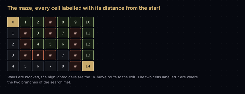
Note that reconstruct was written for string nodes and reused unchanged for (row, column) tuples. A node is whatever you can use as a dictionary key.
How the code maps to the idea
deque is not optional. collections.deque is a doubly linked list of small blocks, so popleft() and append() are both O(1). A list appends in amortised O(1) too, but list.pop(0) shifts every remaining element one slot left: O(n) every time.
visited is checked and set in the same breath. Test membership, add to the set, push to the queue: those three statements are inseparable. Anything reaching queue.append was added to visited on the line above, so nothing else can push it again.
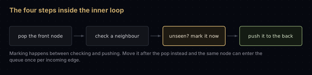
Mark on enqueue, not on dequeue. This is the classic BFS bug, so measure it rather than assert it. The tempting alternative leaves a node unmarked until you pop it. That still terminates and still finds correct distances, provided you skip nodes already processed. What it costs is queue slots.
def enqueues_marking_on_enqueue(graph: dict, source) -> int:
    """The correct version: count how many times anything enters the queue."""
    visited = {source}
    queue = deque([source])
    total = 1

    while queue:
        node = queue.popleft()
        for neighbour in graph[node]:
            if neighbour not in visited:
                visited.add(neighbour)
                queue.append(neighbour)
                total += 1

    return total


def enqueues_marking_on_dequeue(graph: dict, source) -> int:
    """The buggy version: mark on the way out, so a node can be queued twice."""
    visited: set = set()
    queue = deque([source])
    total = 1

    while queue:
        node = queue.popleft()
        if node in visited:
            continue                 # without this guard it re-expands nodes too
        visited.add(node)
        for neighbour in graph[node]:
            if neighbour not in visited:
                queue.append(neighbour)
                total += 1

    return total


print("7-node graph:", enqueues_marking_on_enqueue(graph, "A"),
      "vs", enqueues_marking_on_dequeue(graph, "A"))

# A complete graph on 50 nodes: every node is joined to every other node.
complete = {i: [j for j in range(50) if j != i] for i in range(50)}
print("50-node clique:", enqueues_marking_on_enqueue(complete, 0),
"vs", enqueues_marking_on_dequeue(complete, 0))7-node graph: 7 vs 9
50-node clique: 50 vs 1226Seven versus nine looks harmless. Fifty versus 1,226 does not. Marking on enqueue means a node is pushed at most once, so the queue holds at most V entries ever. Marking on dequeue means it can be pushed once per edge pointing at it, so the queue holds up to O(E). On a sparse graph those are close; on a dense one E is near V², and your O(V) queue has quietly become O(V²).
The source is marked before the loop starts. visited = {source} and parent = {source: None} both do it. Forget it and the source is rediscovered by its own neighbour, pops a second time, and is reported at distance 2 from itself.
parent replaces visited in the shortest-path version. Both answer the same question: has this node been queued?, and keeping two structures in step is two chances to get it wrong. The None parent for the source is what stops reconstruct walking off the end.
Two edge cases fall out for free. A source equal to the target returns a one-node path from the guard at the top. An unreachable target drains the queue without ever matching and returns None, deliberately different from [].
Complexity
Time: O(V + E), with V nodes and E edges. Count the two things BFS does.
Dequeues. A node is appended only in the branch that also adds it to visited, and that branch runs only for nodes not already there. So each node is pushed at most once and popped at most once: V pops, each O(1) from a deque.
Edge scans. When a node pops, the inner loop runs once per entry in its adjacency list: once per edge touching it. Over every popped node that is the sum of all the degrees, which is exactly 2E in an undirected graph, since each edge sits in two lists, and E in a directed one. Each scan is a single set or dict lookup, O(1) on average.
Add them: O(V) + O(2E) = O(V + E). Both terms are needed because either can dominate. A million users with eighty million friendships is edge-heavy; a million nodes with almost no edges is node-heavy.
Best, average and worst are all that same bound for a full traversal. Nothing about the shape of the graph changes the count above: every reachable node is popped once and every edge incident to it is read once, whatever order the adjacency lists happen to be in. The one real best case belongs to bfs_shortest_path, which returns the moment it discovers the target: a target equal to the source returns before the loop starts, and a neighbour of the source costs one pop and one scan of the source's list. That is an early exit, not a cheaper algorithm; miss the target and you are back to the full O(V + E) sweep.
Two caveats. A single BFS only touches the reachable part of the graph, so it costs O(V + E) restricted to that component; the full bound applies when you loop over every node and start a fresh BFS at any still unvisited. And all of this assumes an adjacency list, with an adjacency matrix, listing a node's neighbours means scanning a row of V entries, so BFS becomes O(V²) however few edges there are. That is a large part of why adjacency lists are the default.
Space: O(V). The visited set holds at most V nodes, the parent dictionary at most V entries, and the queue at most V nodes. That queue bound is tight: a star graph — one source joined to V − 1 leaves — puts every leaf in the queue at once the moment the source pops.
That is the real trade against depth-first search. DFS's stack is bounded by the longest path, BFS's queue by the widest level. On a broad, shallow graph (a web crawl, where one page links to a hundred others) BFS holds far more state. On a long, narrow one, DFS does.
When to use it, and when not to
Use BFS when every edge costs the same and you want the fewest of them: minimum moves, fewest hops, degrees of separation, the shortest way through a maze. One traversal hands you every distance from the source at once. It also suits level-ordered work, and it beats recursive DFS on huge graphs because a queue on the heap does not blow Python's recursion limit the way a 100,000-deep call stack does.
Do not use it on a weighted graph. This is the one that bites. A single direct road of 300 km beats a two-hop route of 40 km on edge count and loses badly on distance. For weighted edges use Dijkstra's algorithm, which swaps the FIFO queue for a priority queue keyed on total cost. BFS is exactly Dijkstra with every weight fixed at 1, and in that case the frontier only ever holds two distinct distances, so a plain queue keeps them in order for free and the heap is redundant. If the only weights are 0 and 1, keep the deque and use appendleft for the 0-weight edges: that is 0-1 BFS, still O(V + E).
Do not use it when the graph is broad and memory is tight. A branching factor of 10 puts a million nodes in level 6 alone. Iterative deepening DFS re-explores the shallow levels repeatedly but holds only one path in memory, and for a target far out in a wide graph that trade is often worth it.
Do not use it when you know roughly which way the goal lies. BFS expands equally in every direction, including straight away from the target; A* search biases expansion with a heuristic and can shrink the explored area by orders of magnitude on a map. And when the answer does not depend on distance at all (cycle detection, strongly connected components, articulation points) DFS is the natural tool, since those hang off the shape of the recursion. Topological ordering is the one that goes either way: DFS post-order produces one, and so does Kahn's algorithm, which is a BFS queue driven by in-degree counts.
Where it shows up in the real world
Degrees of separation. LinkedIn's 1st-, 2nd- and 3rd-degree connection labels are BFS levels computed outwards from your profile. Facebook's research team applied the same measure to roughly 1.6 billion users in 2016 and reported an average separation of about 3.57 people. The Erdős number in mathematics and the Bacon number in film are the same thing on co-authorship and co-starring graphs.
Web crawlers. A crawler's frontier is a queue of discovered-but-not-fetched URLs, so taking them in FIFO order is a breadth-first crawl. Najork and Wiener showed in 2001 that crawling breadth-first tends to pull in high-PageRank pages early, which matters when you can only fetch a fraction of the web.
Flood fill. The paint-bucket tool in an image editor is BFS over pixels, with "same colour as the pixel I clicked" as the edge condition, and Minesweeper's cascade over blank squares is the same traversal. BFS is preferred to recursive DFS here because a large region would overflow the call stack.
Copying garbage collectors. Cheney's algorithm walks the live object graph breadth-first, using the space it is copying into as the queue itself: objects already copied but not yet scanned sit between two pointers. It needs no separate stack at all.
Maximum flow. Edmonds-Karp is Ford-Fulkerson with one change: find each augmenting path with BFS. Picking the path with the fewest edges is exactly what bounds the iteration count and gives the guaranteed O(V·E²).
Python's standard library has no BFS of its own; what it gives you is collections.deque, the queue you build it on. If you have networkx available, nx.shortest_path(G, source, target) with no weight argument runs a bidirectional BFS: two searches, one from each end, meeting in the middle.
Common mistakes
Marking visited when you pop instead of when you push. The one measured above. The traversal still works, but a node can be queued once per incoming edge, so the queue grows from O(V) to O(E): 1,226 pushes instead of 50 on a 50-node clique. Mark a node the instant you decide to queue it.
Using a list as the queue. queue.pop(0) on a list is O(n), because every remaining element shifts down one slot. That turns an O(V + E) algorithm into an O(V² + E) one for nothing. Use collections.deque and popleft().
Forgetting to mark the source. If visited starts empty rather than holding the source, the source's own neighbour rediscovers it, pushes it again, and it comes back out of the queue reported as two edges from itself.
Running BFS on weighted edges. BFS counts hops. If your edges carry costs, times or distances, the fewest-hop path can be arbitrarily worse than the cheapest one. Reach for Dijkstra instead.
Forgetting to reverse the reconstructed path. Parent pointers run from the target back to the source, so the raw walk gives the route backwards. Reverse it, and check the length: a path of k edges holds k + 1 nodes, which is why 14 moves through the maze printed a path length of 15.
Practice
- Return every node exactly
kedges from a source, usingbfs_levelsand nothing else. - Count the connected components of an undirected graph by starting a fresh BFS at every node still unvisited.
- Implement multi-source BFS: seed the queue with several starting cells at distance 0 at once, and label every cell of a grid with its distance to the nearest exit.
- Decide whether a graph is bipartite by colouring each node by the parity of its BFS level and checking that no edge joins two nodes of the same colour.
- Write bidirectional BFS (alternate a level of expansion from the source with one from the target, stopping when the frontiers touch), and count how many nodes each version pops on a long chain graph.
Summary
BFS is a queue, a visited set, and the discipline to mark nodes on the way in rather than on the way out. That discipline buys a traversal where each node is dequeued once and each edge read once per endpoint, which is where O(V + E) comes from, plus an ordering by distance that makes the first arrival at any node provably the shortest. Everything else (level grouping, path reconstruction, mazes, flood fill) is the same nine-line loop wearing different clothes.
| Difficulty | Medium |
| Time | O(V + E) — every node leaves the queue once, every edge is read once per endpoint |
| Best / worst case | Both O(V + E) for a full traversal; only the shortest-path version's early exit can stop sooner |
| Time (adjacency matrix) | O(V²) — listing one node's neighbours costs a full row scan |
| Space | O(V) — visited set, parent map, and a queue that never spans more than two adjacent levels |
| Graph type | Unweighted; directed or undirected, cyclic or acyclic |
| Finds shortest path | Yes — shortest in edges, not in weight |
| Handles cycles | Yes — the visited set stops any node being expanded twice |
| Complete | Yes — finds a path if one exists, on any finite graph |
| Data structure | FIFO queue (collections.deque) over an adjacency list |
| Use it when | Fewest-hop paths, level ordering, connectivity, flood fill, multi-source distance |
| Avoid it when | Edges are weighted (use Dijkstra), the graph is very broad, or a good heuristic exists |
| Real-world use | LinkedIn connection degrees, web crawl frontiers, flood fill, Cheney GC, Edmonds-Karp |
| Python equivalent | None in the standard library; collections.deque is the queue you build it on |
Learn BFS properly and three later algorithms cost you almost nothing: Dijkstra is BFS with a priority queue, A* is Dijkstra with a heuristic, and Edmonds-Karp is a max-flow algorithm whose one clever idea is to pick augmenting paths with BFS. The queue is the part you should be able to write from memory.
Keep reading
- Graphs in Python — adjacency lists versus matrices, and why the choice changes BFS's complexity.
- Depth-First Search — the same traversal with a stack instead of a queue, and the problems it is better at.
- Dijkstra's Algorithm — what to do when the edges have weights and hop counting stops working.
- Queues and Deques in Python — why
collections.dequeis O(1) at both ends and a list is not. - Topological Sort — Kahn's algorithm is BFS over a dependency graph, driven by in-degree instead of distance.


