
Breadth-first search finds the shortest path in a graph where every edge costs the same. Real maps are not like that. One road is 400 metres of clear tarmac and the next is 400 metres of roadworks; one network link is a gigabit fibre and the next is a saturated DSL line. As soon as edges carry different weights, "fewest hops" and "cheapest route" stop being the same question, and BFS answers the wrong one.
Dijkstra's algorithm answers the right one. It is a single greedy rule repeated until the graph runs out: always expand the unfinished node you can currently reach most cheaply, and use it to improve your estimate for its neighbours. That rule rests on one invariant (the moment a node is pulled off the queue, its distance is final and will never change again), and everything interesting about the algorithm follows from that invariant, including its speed and its one hard limitation.
The limitation is negative edge weights, and it is not a bug you can patch. This post works through the counterexample by hand so you can see the invariant break rather than take somebody's word for it. Along the way: a full trace on a six-node graph, an implementation on heapq using the lazy-deletion pattern, predecessor tracking so you get the actual route and not just its cost, and the counting argument behind O((V + E) log V).
The idea
You are given a graph, a starting node, and a weight on every edge. The weight is a cost: distance, minutes, latency, money. You want the cheapest total cost from the start to every other node.
Keep two things for every node: a tentative distance (the cheapest route to it you have found so far, starting at infinity for everything except the source, which is 0) and a flag for whether it is settled. Settled means finished — the tentative distance has been promoted to the true shortest distance and will not be touched again.
The core operation is relaxation. If you know you can reach u for a cost of 7, and there is an edge from u to v weighing 3, then you can reach v for 10. If your current estimate for v is worse than 10, replace it. That is the whole operation: one addition and one comparison.
The greedy choice is what turns relaxation into an algorithm:
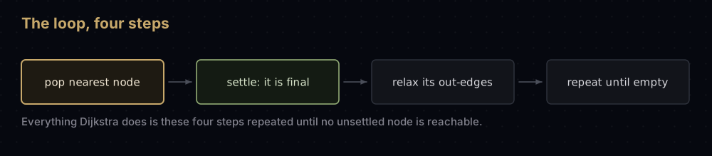
Among all unsettled nodes, take the one with the smallest tentative distance and settle it. Then relax every edge leaving it. Repeat until there is nothing left to settle.
Why is it safe to declare that node finished? Suppose you settle u at distance d, and some cheaper path to u exists that you have not found. That path starts at the source, which is settled, and ends at u, which is not, so somewhere along it there is a first step from a settled node into an unsettled node y. You have already relaxed that edge, so your estimate for y is at most the cost of the path up to y. The rest of the path, from y onwards, can only add cost and never remove it, so the whole path costs at least your estimate for y. But you chose u because it had the smallest estimate, so the estimate for y is at least d. The "cheaper" path therefore costs at least d. It was never cheaper.
Read that argument again and notice exactly where it leans on the weights. "The rest of the path can only add cost and never remove it" is true only if no edge is negative. That one clause is the entire reason Dijkstra cannot handle negative weights, and there is a three-node graph below that shows it failing.
Watching it work
Six nodes, nine directed edges, starting from A:
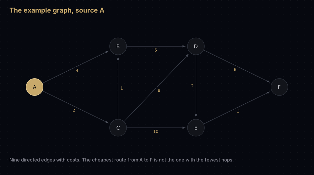
Distances start at 0 for A and infinity for everything else. Now settle nodes one at a time, smallest estimate first.
Settle A at 0. Relax its two edges. B becomes 4, C becomes 2.
Settle C at 2 — it is the smallest unsettled estimate, beating B's 4. Relax C's edges: B improves from 4 to 3 (2 + 1), D becomes 10 (2 + 8), E becomes 12 (2 + 10). Notice that B just got cheaper after it already had a value. That is normal, and it is only allowed because B was still unsettled.
Settle B at 3. Relax B to D: 3 + 5 = 8, which beats the 10 that came through C. D drops to 8.
Settle D at 8. Relax D to E: 8 + 2 = 10, beating 12. Relax D to F: 8 + 6 = 14.
Settle E at 10. Relax E to F: 10 + 3 = 13, beating 14.
Settle F at 13. It has no outgoing edges. Every node is settled, and the algorithm stops.
Here is every value the distance table ever holds:
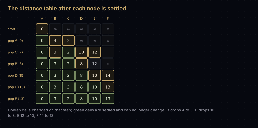
The order in which nodes were settled (A, C, B, D, E, F at 0, 2, 3, 8, 10, 13) is sorted by distance. That is not a coincidence; it is forced by the greedy rule, and it is why Dijkstra can stop early if you only care about one destination.
The costs are only half the answer. If you also record, for each node, which node improved it last, you get the route for free:
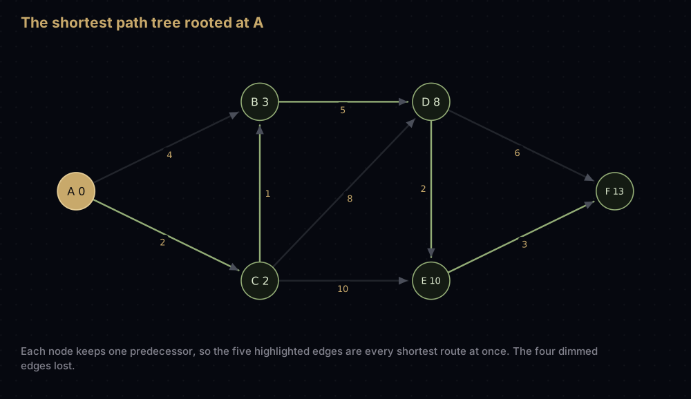
Five nodes each have one predecessor, so the shortest routes form a tree rooted at A. Follow F's predecessor chain backwards: F came from E, E from D, D from B, B from C, C from A. Reverse it and you get A → C → B → D → E → F, which costs 2 + 1 + 5 + 2 + 3 = 13. The direct-looking route A → B → D → F costs 4 + 5 + 6 = 15 and loses.
The code
Start with the graph. An adjacency list — each node mapped to its outgoing (target, weight) pairs — is the right shape here, because the inner loop only ever asks "what leaves this node?".
The simplest correct implementation does not use a heap at all. It finds the nearest unsettled node by scanning the whole distance table.
from __future__ import annotations

import heapq

# A weighted directed graph: every node maps to its outgoing (target, weight)
# pairs. Nodes with no outgoing edges still need a key, or they vanish.
Graph = dict[str, list[tuple[str, int]]]

roads: Graph = {
    "A": [("B", 4), ("C", 2)],
    "B": [("D", 5)],
    "C": [("B", 1), ("D", 8), ("E", 10)],
    "D": [("E", 2), ("F", 6)],
    "E": [("F", 3)],
    "F": [],
}


def dijkstra_scan(graph: Graph, source: str) -> dict[str, float]:
    """Shortest distance from source to every node, choosing the next node
    by scanning the whole distance table.

    No heap, no duplicate bookkeeping. This is the O(V^2) version, and it is
    the one to prefer when the graph is dense.
    """
    distances: dict[str, float] = {node: float("inf") for node in graph}
    distances[source] = 0
    settled: set[str] = set()

    while len(settled) < len(graph):
        # The nearest unsettled node: nothing can reach it more cheaply, so
        # its tentative distance is now final.
        current = min((node for node in graph if node not in settled),
                      key=lambda node: distances[node])
        if distances[current] == float("inf"):
            break  # the rest of the graph is unreachable from source
        settled.add(current)

        for neighbour, weight in graph[current]:
            if neighbour in settled:
                continue
            candidate = distances[current] + weight
            if candidate < distances[neighbour]:
                distances[neighbour] = candidate

    return distances


print(dijkstra_scan(roads, "A")){'A': 0, 'B': 3, 'C': 2, 'D': 8, 'E': 10, 'F': 13}That min(...) call is the bottleneck: it walks every node on every iteration. Replace it with a binary heap and the same algorithm gets a much better bound on sparse graphs. Python's heapq module is that heap: it turns a plain list into a min-heap where heappush and heappop both cost O(log n).
There is one wrinkle. Textbook Dijkstra says "decrease the key of v in the priority queue". heapq has no decrease_key, because a list-backed heap cannot find an arbitrary element without scanning it. The idiomatic fix, and the one the heapq documentation itself recommends, is lazy deletion: never update an entry, just push a new one, and throw away entries that are already out of date when you pop them.
def dijkstra(graph: Graph, source: str) -> tuple[dict[str, float], dict[str, str | None]]:
    """Shortest distances and predecessors from source, using a binary heap.

    Instead of decreasing a key inside the heap, an improved node is pushed
    again. Any later entry for a node already settled is stale and skipped,
    so the heap holds at most one entry per relaxation that improved
    something.
    """
    distances: dict[str, float] = {node: float("inf") for node in graph}
    distances[source] = 0
    previous: dict[str, str | None] = {node: None for node in graph}
    settled: set[str] = set()
    heap: list[tuple[float, str]] = [(0, source)]

    while heap:
        distance, node = heapq.heappop(heap)
        if node in settled:
            continue  # stale duplicate: a cheaper entry for it popped earlier
        settled.add(node)

        for neighbour, weight in graph[node]:
            if neighbour in settled:
                continue  # its distance is final; nothing here can beat it
            candidate = distance + weight
            if candidate < distances[neighbour]:
                distances[neighbour] = candidate
                previous[neighbour] = node
                heapq.heappush(heap, (candidate, neighbour))

    return distances, previous


distances, previous = dijkstra(roads, "A")
for node in sorted(distances):
print(f"{node}: distance {distances[node]}, reached from {previous[node]}")A: distance 0, reached from None
B: distance 3, reached from C
C: distance 2, reached from A
D: distance 8, reached from B
E: distance 10, reached from D
F: distance 13, reached from EThe previous dictionary is the whole route, stored in one entry per node. Walking it backwards and reversing gives the path:
def reconstruct_path(previous: dict[str, str | None], source: str, target: str) -> list[str]:
    """Walk the predecessor chain backwards from target, then reverse it."""
    if target != source and previous.get(target) is None:
        return []  # unreachable from source, or not in the graph at all

    path = [target]
    while path[-1] != source:
        path.append(previous[path[-1]])
    path.reverse()
    return path


for node in sorted(distances):
    route = " -> ".join(reconstruct_path(previous, "A", node))
    print(f"cost {distances[node]:>2}   {route}")

islands: Graph = {"X": [("Y", 3)], "Y": [], "Z": []}
island_distances, island_previous = dijkstra(islands, "X")
print("Z:", island_distances["Z"], reconstruct_path(island_previous, "X", "Z"))cost 0 A
cost 3 A -> C -> B
cost 2 A -> C
cost 8 A -> C -> B -> D
cost 10 A -> C -> B -> D -> E
cost 13 A -> C -> B -> D -> E -> F
Z: inf []How the code maps to the idea
distances is the tentative-distance table from the walkthrough, and float("inf") is the honest starting value: no route is known yet. Python's inf compares correctly with every number, so candidate < distances[neighbour] is true the first time any real route is found, without a special case for "unset".
settled is the finished set. Adding a node to it is the moment the invariant fires: that node's distance is now final. Everything else in the loop exists to make sure nothing is settled too early.
The heap holds (distance, node) tuples in that order because Python compares tuples left to right, so the smallest distance always sits at the root. Putting the node first would sort alphabetically and quietly break the algorithm.
The stale check is the two lines that make lazy deletion work. When a node improves, a fresh entry is pushed and the old, worse entry stays in the heap. Because the old entry has a larger distance, it is guaranteed to pop later than the good one: by which time the node is in settled, so continue discards it. The heap can hold several entries for one node; at most one of them is ever acted on.
Here is the same algorithm printing every pop, so the discarded entries are visible:
def dijkstra_traced(graph: Graph, source: str) -> None:
    """Same algorithm, printing every pop so the stale entries are visible."""
    distances: dict[str, float] = {node: float("inf") for node in graph}
    distances[source] = 0
    settled: set[str] = set()
    heap: list[tuple[float, str]] = [(0, source)]

    while heap:
        distance, node = heapq.heappop(heap)
        if node in settled:
            print(f"skip {node} @ {distance:<4} stale: {node} was settled at {distances[node]}")
            continue
        settled.add(node)
        print(f"pop  {node} @ {distance:<4} settled, distance is final")

        for neighbour, weight in graph[node]:
            if neighbour in settled:
                continue
            candidate = distance + weight
            if candidate < distances[neighbour]:
                print(f"        relax {node}->{neighbour}: {distances[neighbour]} becomes {candidate}, push ({candidate}, {neighbour!r})")
                distances[neighbour] = candidate
                heapq.heappush(heap, (candidate, neighbour))


dijkstra_traced(roads, "A")pop A @ 0 settled, distance is final
relax A->B: inf becomes 4, push (4, 'B')
relax A->C: inf becomes 2, push (2, 'C')
pop C @ 2 settled, distance is final
relax C->B: 4 becomes 3, push (3, 'B')
relax C->D: inf becomes 10, push (10, 'D')
relax C->E: inf becomes 12, push (12, 'E')
pop B @ 3 settled, distance is final
relax B->D: 10 becomes 8, push (8, 'D')
skip B @ 4 stale: B was settled at 3
pop D @ 8 settled, distance is final
relax D->E: 12 becomes 10, push (10, 'E')
relax D->F: inf becomes 14, push (14, 'F')
skip D @ 10 stale: D was settled at 8
pop E @ 10 settled, distance is final
relax E->F: 14 becomes 13, push (13, 'F')
skip E @ 12 stale: E was settled at 10
pop F @ 13 settled, distance is final
skip F @ 14 stale: F was settled at 13Six real pops and four discarded ones. Every discarded entry is a relaxation that was later beaten by a better one, and skipping it costs a single set lookup.
Why prefer this to a real decrease-key? Three reasons, and the first is decisive. heapq does not expose one, so implementing it means writing your own heap plus a node-to-index map updated inside every sift step: dozens of lines of Python instead of two, and none of them running in the C that backs heapq. Second, the asymptotic cost is the same: lazy deletion makes the heap hold up to E entries instead of V, and log(V²) is 2 log V, so the log factor is unchanged. Third, the extra pops are cheap; each one is a heappop and a set membership test.
Edge cases fall out of the structure. A node unreachable from the source is never pushed, keeps its inf, and reconstruct_path returns an empty list for it. That is the Z: inf [] line above. A source with no outgoing edges settles itself and the loop ends. A self-loop of weight 0 or more never improves anything, so it is ignored. Parallel edges between the same pair are fine, because relaxation keeps whichever is cheapest.
Why a negative edge breaks it
Take three nodes. A to B costs 2. A to C costs 5. C to B costs -4.
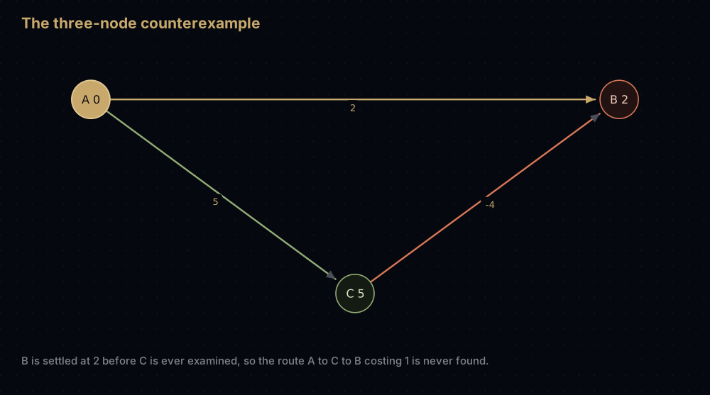
Run the algorithm in your head. A settles at 0 and relaxes both edges: B becomes 2, C becomes 5. The smallest unsettled estimate is now B at 2, so B is settled at 2 and never looked at again. Then C settles at 5, and its edge to B would give 5 + (-4) = 1 — a genuinely better route — but B is finished. The answer comes out as 2 when the truth is 1.
detour: Graph = {
    "A": [("B", 2), ("C", 5)],
    "B": [],
    "C": [("B", -4)],
}

broken, broken_previous = dijkstra(detour, "A")
print("dijkstra:", broken["B"], "via", reconstruct_path(broken_previous, "A", "B"))
print("truth:   ", 5 + -4, "via ['A', 'C', 'B']")

detour_plus: Graph = dict(detour, B=[("D", 1)], D=[])
broken_plus, _ = dijkstra(detour_plus, "A")
print("with D behind B:", broken_plus["D"], "instead of", 5 + -4 + 1)dijkstra: 2 via ['A', 'B']
truth: 1 via ['A', 'C', 'B']
with D behind B: 3 instead of 2Nothing crashes and nothing warns. The function returns a cost of 2 and a route of A → B, both internally consistent and both wrong. The better route is never even considered: by the time C is settled, B is in settled, so the relaxation of the edge C to B is skipped outright. This is the failure mode that survives a test suite built on graphs where every weight happens to be positive.
The third line shows how far the damage spreads. Put a node D behind B, one step past it at weight 1, and Dijkstra reports 3 for D because D was expanded from B's wrong value of 2. Patching B's number afterwards would not help on its own: nothing recomputes D. The error propagates forward through everything that was routed through the node you settled too early.
You can get correct answers back by dropping the settled check and re-pushing any node whose distance improves; on this graph that works. What it costs is the bound. Once a node can be expanded more than once, graphs exist on which the number of expansions grows exponentially with the number of nodes, which is why negative weights call for a different algorithm rather than a patched Dijkstra.
Note that this graph has no negative cycle. The shortest path is perfectly well defined; Dijkstra just cannot find it. When weights can be negative, use Bellman-Ford, which relaxes every edge V − 1 times in O(V · E) and detects negative cycles as a bonus. For all-pairs shortest paths with negative edges, use Floyd-Warshall.
One tempting "fix" deserves killing off: adding a constant to every weight to make them all non-negative does not work. It penalises paths with more edges, because a path of 5 edges absorbs the constant five times and a path of 2 edges absorbs it twice. You will get a shortest path for a different problem.
Complexity
Count the operations rather than quoting the letters.
Each node is settled at most once. The settled set guarantees it. So across the entire run, the inner for loop runs once per node's adjacency list, and every edge in the graph is examined exactly once from its tail. That is E relaxation attempts in total, plus O(V) for setting up the tables.
Each successful relaxation pushes exactly one heap entry, and a relaxation can only succeed on an edge it is examining. So there are at most E pushes, plus 1 for the source. Pops cannot exceed pushes, so at most E + 1 pops.
Each push and pop costs O(log H) where H is the heap size, and H never exceeds E + 1. In a simple graph E is at most V(V − 1), so log E is at most 2 log V. Constant factors vanish in big O, so log E is O(log V).
Multiply out: O(V) setup + O(E) edge scans + O(E) heap operations at O(log V) each, giving O(V + E log V), conventionally written O((V + E) log V). On a sparse graph like a road network, where each junction has a handful of roads and E is roughly proportional to V, that is effectively O(V log V).
The array-scan version is O(V²). It settles V nodes and scans all V entries each time to find the minimum, so V² work in the scans, plus E relaxations that are O(1) each: O(V² + E), and since E ≤ V² that is O(V²). Compare the two on a dense graph where E is about V²: the heap version costs V² log V and the scan version costs V². The scan version wins on dense graphs, and this is a real result, not a technicality: if you are running shortest paths on an adjacency matrix, the simpler code is also the faster one.
Fibonacci heaps give O(E + V log V), which is asymptotically better because decrease-key becomes O(1) amortised and only the V extract-min operations pay the log. In practice they are slower than a binary heap on anything but enormous graphs, because their constant factors and pointer chasing are brutal. Know that the bound exists; do not implement one.
Space is O(V + E). The distance table, predecessor table and settled set are one entry per node. The heap is the extra cost of lazy deletion: up to E + 1 entries rather than the V a decrease-key implementation would hold. The adjacency list itself is O(V + E).
There is no meaningful best case. Dijkstra must settle every reachable node before it can be sure about the furthest one, so it always does the full work unless you only want one destination, in which case you can stop the moment that node pops and skip every node further away than it.
When to use it, and when not to
Use it when edges have non-negative weights and you need exact cheapest routes from one source. This is the default choice for weighted shortest paths, and there is rarely a reason to reach for anything else in that situation.
Do not use it when all edges have the same weight. Breadth-first search gives the same answer in O(V + E) with a collections.deque and no heap. Dijkstra on an unweighted graph is just BFS with unnecessary logarithms.
Do not use it when any weight can be negative. Use Bellman-Ford, as above.
Do not use it when you have a good estimate of the remaining distance to a single target: straight-line distance on a map, for instance. A* search is Dijkstra with that estimate added to the priority, and on a road network it explores a small fraction of the nodes because it stops fanning out in every direction.
Do not use it when you need distances between every pair of nodes in a dense graph. Running Dijkstra V times costs O(V · (V + E) log V); Floyd-Warshall does it in O(V³) with three tight loops and no data structures at all.
Do not use it when you want to connect every node as cheaply as possible rather than to reach them cheaply from one start. That is a minimum spanning tree, and Prim's algorithm looks almost identical to Dijkstra: the only difference is that the heap key is the edge weight alone, not the accumulated distance.
Where it shows up in the real world
Link-state routing protocols. OSPF (RFC 2328) and IS-IS both work by flooding every router's local link state to the whole area, so each router builds an identical map of the topology, and then each one independently runs Dijkstra over that map to compute its own forwarding table. The literature calls this the SPF — shortest path first — calculation. They are the two dominant interior gateway protocols on large networks, and every router in an area re-runs its SPF calculation whenever a link changes state.
Map and journey routing. Dijkstra is the correctness baseline for road navigation, and production routers are built on top of it rather than replacing it. Open Source Routing Machine (OSRM) and similar engines precompute contraction hierarchies so that a query touches a tiny part of the graph, but the query itself is still a bidirectional Dijkstra search over the contracted graph. Public-transport routers layer timetable constraints over the same relaxation loop.
Game pathfinding. A* is the usual per-unit choice, but when many units head for the same destination, engines run one Dijkstra from that destination across the whole navigation grid and cache the result as a flow field or "Dijkstra map"; each unit then just walks downhill. One search serves a hundred units.
Scientific and general-purpose libraries. scipy.sparse.csgraph.dijkstra and NetworkX's shortest_path are the two you are most likely to call from Python. Neither accepts a plain dictionary of lists: SciPy wants the graph as a sparse adjacency matrix, NetworkX wants one of its own graph objects, so converting the shape used above is the first step in both cases.
Common mistakes
Settling a node when you push it instead of when you pop it. This is the classic Dijkstra bug. Add the neighbour to settled at push time and its distance is frozen at the first value anyone happened to find, not the smallest. On the example graph B would be marked finished at 4 the moment A relaxed into it, so the 3 arriving later through C would be thrown away and D, E and F would all inherit the error. A node is only final when it comes out of the heap.
Not skipping stale heap entries. Without the if node in settled: continue line, a node gets expanded once per heap entry it accumulated. With non-negative weights the answers still come out right — a stale entry's larger distance produces candidates that fail the < test — but each one re-walks a whole adjacency list for nothing.
Putting the node first in the tuple. (node, distance) sorts alphabetically, which turns the priority queue into an alphabetiser. Nothing crashes; the output is just wrong.
Forgetting nodes with no outgoing edges. If your adjacency list only has keys for nodes that have edges, then graph[node] raises KeyError on a dead end and distances is missing entries. Either build the dictionary with every node as a key, as above, or use graph.get(node, []).
Running it on negative weights anyway. The failure is silent, plausible-looking, and only shows up on the inputs where it matters.
Rebuilding the whole heap to simulate decrease-key. Calling heapify after editing the list is O(n) per update and turns the algorithm into something worse than the O(V²) scan version. Push a duplicate instead.
Practice
- Add a
targetparameter that returns as soon as that node is popped, and count how many fewer pops the six-node example needs when you ask only for D. - Make the graph undirected by adding the reverse of every edge, then work out why not one of the distances from A changes.
- Return the number of distinct shortest paths to each node as well as the distance, by adding a counter that resets on an improvement and accumulates on a tie.
- Modify the algorithm to maximise the bottleneck instead: find the route from A to F whose narrowest edge is as wide as possible, by replacing the addition with a minimum and the comparison with a maximum.
- Write a checker that runs both
dijkstra_scananddijkstraon 200 randomly generated graphs with a fixed seed and asserts the distance tables match.
Summary
Dijkstra's algorithm is one greedy rule and one invariant: settle the nearest unsettled node, and trust that its distance is final. That invariant is what makes the algorithm fast, and it is precisely what a negative edge destroys: a cheaper route can arrive after the node has already been closed, and nothing goes back to fix it. In Python, build it on heapq with lazy deletion rather than fighting for a decrease-key, keep a previous table so you get routes and not just costs, and drop to the O(V²) scan when the graph is dense.
| Difficulty | Hard |
| Time, binary heap | O((V + E) log V) — at most E + 1 pushes and pops, each O(log E), and log E ≤ 2 log V |
| Time, array scan | O(V²) — V minimum-scans over V nodes; faster when E approaches V² |
| Time, Fibonacci heap | O(E + V log V) — theoretically better, slower in practice |
| Space | O(V + E) — three tables of size V, plus up to E + 1 heap entries |
| Graph type | Directed or undirected, weighted, non-negative weights only |
| Handles negative weights | No — the settled-is-final invariant fails; use Bellman-Ford |
| Detects negative cycles | No |
| Returns | Distance from one source to all nodes, plus a shortest-path tree |
| Use it when | Weights differ, weights are non-negative, and you need exact routes |
| Avoid it when | Weights are uniform (use BFS), negative (Bellman-Ford), or you have a heuristic (A*) |
| Real-world use | OSPF and IS-IS routing, road and transit navigation, game flow fields |
| Python equivalent | None in the standard library; heapq supplies the queue, scipy.sparse.csgraph.dijkstra if a dependency is acceptable |
Keep reading
- Breadth-First Search — the unweighted case, and the algorithm Dijkstra collapses into when every edge costs 1.
- Bellman-Ford — what to run when a weight can be negative, and how it detects negative cycles.
- A* Search — the same loop plus a heuristic, and why that makes map routing practical.
- Heaps and Priority Queues — how
heapqgets O(log n) pushes and pops, from the sift operations up. - Graphs in Python — adjacency lists versus matrices, and why the choice decides which Dijkstra to write.


