Dijkstra's algorithm and Bellman-Ford answer one question: what is the cheapest route from this vertex to everywhere else. Floyd-Warshall answers a different one. Hand it a graph with V vertices and it fills in a complete V by V table — the cheapest route from every vertex to every other vertex — in a single run.
What makes it worth learning is how little machinery it needs to do that. No priority queue. No visited set. No traversal, no recursion, no frontier of any kind. Three nested loops over a grid of numbers, and the body of the innermost loop is one addition, one comparison and one assignment.
The catch is the loop order. The three loops are not interchangeable. Get the order wrong and the code still compiles, still runs, still returns a full table of plausible-looking numbers, and the numbers are wrong. That detail is most of what there is to understand here, so it gets most of the attention below.
The idea
Forget graph traversal for a moment and think about a table.
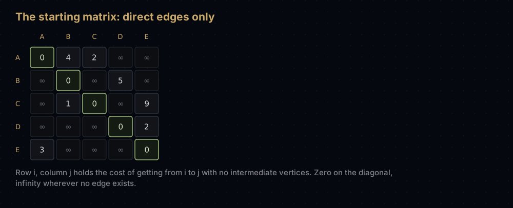
Number the vertices 0 to V − 1 and keep a V by V grid called dist, where dist[i][j] is the cheapest route from i to j that you currently know about. Fill it in with what you can read straight off the graph and nothing more: dist[i][i] = 0, because staying put is free; dist[i][j] = w when an edge of weight w runs from i to j; and infinity everywhere else, meaning "no route known".
That table already answers one very restricted question correctly: what is the cheapest route that uses no intermediate vertices at all? Floyd-Warshall's entire job is to lift that restriction, one vertex at a time.
Pick a vertex k. For every pair of vertices i and j, ask one question: is going from i to j via k cheaper than the best route you already know? The answer is arithmetic.
if dist[i][k] + dist[k][j] < dist[i][j]:
    dist[i][j] = dist[i][k] + dist[k][j]
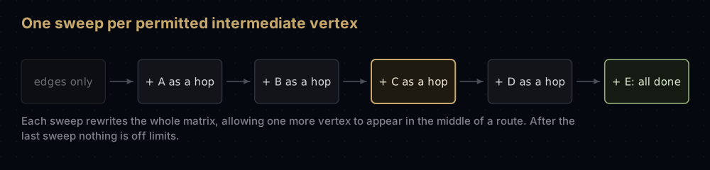
Do that for all V² pairs. Then pick the next k and sweep the whole table again. After every vertex has had a turn as k, the table holds true shortest-path costs.
Why that works: it is dynamic programming
Write D0 for the table where routes get no intermediate vertices at all: the one you just filled in from the edge list. Write D1 for the table where routes may pass through vertex 0 and nothing else. Any route from i to j in D1 either uses vertex 0 or it does not. If it does not, its cost is D0[i][j]. If it does, it splits at vertex 0 into an i-to-0 leg and a 0-to-j leg, neither of which may use vertex 0 in the middle, so its cost is D0[i][0] + D0[0][j]. Take the cheaper of the two:
D1[i][j] = min( D0[i][j], D0[i][0] + D0[0][j] )Nothing there was special to vertex 0. Run the argument again to build D2 from D1 by permitting vertex 1, then D3 from D2, and so on: Dk+1[i][j] is the smaller of Dk[i][j] and Dk[i][k] + Dk[k][j]. After V layers every vertex is permitted, "restricted" means "unrestricted", and DV is the answer.
One subtlety hides in "it splits at vertex 0". A route could visit vertex 0 twice, and then the split is not clean. But a route that revisits a vertex contains a cycle, and provided no cycle has negative total weight, deleting that cycle never makes the route more expensive. So some optimal route repeats no vertex, and "via k" safely means "via k exactly once". Dijkstra and Bellman-Ford rest on the same fact, and it is precisely what negative cycles destroy.
Why k has to be the outer loop
To compute any cell of layer k + 1 you need three finished numbers from layer k: Dk[i][j], Dk[i][k] and Dk[k][j]. The last two range over every i and every j, so the entire row k and the entire column k of layer k must be complete before you touch a single cell of layer k + 1. Only one nesting guarantees that: k on the outside, one full sweep of the matrix per value of k.
Put k innermost and you are asking, for one pair in isolation, "what is the best route through 0, then through 1, then through 2…", reading row and column values that do not exist yet. Sometimes it lands on the right answer. Often it does not — there is a demonstration further down where the wrong order reports two pairs as unreachable that are comfortably reachable.
The i and j loops, by contrast, are freely interchangeable. Within a single value of k, no cell the body reads is ever written.
One matrix, not V of them
The recurrence describes V + 1 separate tables, but implementations keep one and overwrite it in place. That is safe, and it is where the O(V²) space bound comes from.
During sweep k, could the body overwrite dist[i][k], a value the rest of the sweep still depends on? Only if dist[i][k] + dist[k][k] were strictly smaller than dist[i][k], which needs dist[k][k] to be negative. It starts at 0 and only drops below 0 once the graph has a negative cycle. The same argument covers dist[k][j]. So row k and column k are frozen for the whole sweep, every read returns the layer-k value the recurrence demands, and one matrix does the work of V + 1.
Watching it work
Here is a five-vertex directed graph. The vertices are numbered 0 to 4 in the code and named A to E here so the trace reads more easily.
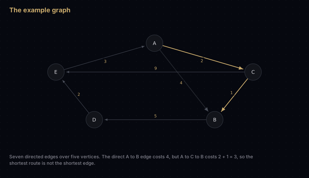
The seven edges, written as source, target, weight:
A -> B  4        C -> B  1        E -> A  3
A -> C  2        C -> E  9
B -> D  5        D -> E  2
Read into a matrix, before the algorithm touches anything:
Sweep k = A. Only one row has a finite entry in column A: dist[E][A] = 3, the edge E to A. Everywhere else that column is infinity, and infinity plus anything is infinity, so only row E can gain. It gains two cells — E to B at 3 + 4 = 7, and E to C at 3 + 2 = 5.
Sweep k = B. Column B now holds 4 from A, 1 from C and 7 from E, and row B holds one useful entry, the edge B to D of weight 5. Three cells improve, all in column D: A to D at 4 + 5 = 9, C to D at 1 + 5 = 6, E to D at 7 + 5 = 12.
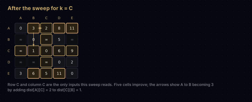
Sweep k = C. This is the sweep that earns the algorithm its keep. Row C reads 1 to B, 6 to D (computed one sweep ago) and 9 to E; column C reads 2 from A and 5 from E. Five cells improve, and one is the headline: dist[A][B] drops from 4 to 3, because the direct edge A to B costs 4 while A to C to B costs 2 + 1 = 3. The rest are A to D falling 9 to 8, A to E appearing at 2 + 9 = 11, E to B falling 7 to 6, and E to D falling 12 to 11.
Sweep k = D. Row D offers one thing, the edge D to E of weight 2, so this sweep only ever writes into column E. A to E falls from 11 to 8 + 2 = 10, B to E appears at 5 + 2 = 7, and C to E falls from the direct edge's 9 to 6 + 2 = 8.
Sweep k = E. Column E is full by now and row E reads 3 to A, 6 to B, 5 to C, 11 to D. This sweep fills the entire bottom-left of the table: B to A at 7 + 3 = 10, B to C at 7 + 5 = 12, C to A at 8 + 3 = 11, and all of row D, previously empty apart from D to E (D to A at 2 + 3 = 5, D to B at 2 + 6 = 8, D to C at 2 + 5 = 7).
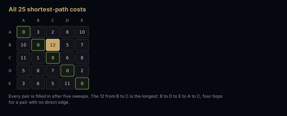
Nineteen writes landed across the five sweeps, touching fifteen distinct cells. Notice what the last sweep did: before it, most of the lower half of the matrix still said "unreachable", because every route out of B, C or D back to A must pass through E, and E was the last vertex permitted as an intermediate. Number the vertices differently and a different sweep fixes each cell; the final table is identical either way.
The code
Start with reading a graph into a matrix. float("inf") is the right sentinel here: it compares greater than every real number, and adding anything to it gives infinity back, so the relaxation line needs no special cases at all.
from __future__ import annotations  # lets `int | None` work on older Pythons

INF = float("inf")

NAMES = "ABCDE"
EDGES: list[tuple[int, int, float]] = [
    (0, 1, 4),  # A -> B
    (0, 2, 2),  # A -> C
    (1, 3, 5),  # B -> D
    (2, 1, 1),  # C -> B
    (2, 4, 9),  # C -> E
    (3, 4, 2),  # D -> E
    (4, 0, 3),  # E -> A
]


def build_matrix(vertex_count: int,
                 edges: list[tuple[int, int, float]]) -> list[list[float]]:
    """Turn an edge list into a V by V distance matrix.

    Every pair starts at infinity, the diagonal starts at zero because staying
    put is free, and parallel edges collapse to the cheapest one.
    """
    dist = [[INF] * vertex_count for _ in range(vertex_count)]
    for vertex in range(vertex_count):
        dist[vertex][vertex] = 0.0
    for source, target, weight in edges:
        dist[source][target] = min(dist[source][target], weight)
    return dist


def cell(value: float) -> str:
    """Format one entry for printing; a dot means 'no route known'."""
    return "." if value == INF else str(int(value))


def show(dist: list[list[float]], title: str, names: str = NAMES) -> None:
    print(title)
    print("     " + "".join(f"{name:>5}" for name in names))
    for index, row in enumerate(dist):
        print(f"{names[index]:>5}" + "".join(f"{cell(value):>5}" for value in row))


show(build_matrix(5, EDGES), "direct edges only")direct edges only
A B C D E
A 0 4 2 . .
B . 0 . 5 .
C . 1 0 . 9
D . . . 0 2
E 3 . . . 0The algorithm itself is the three loops, and that is the whole of it.
def floyd_warshall(dist: list[list[float]]) -> list[list[float]]:
    """All-pairs shortest paths, rewriting `dist` in place.

    After the outer loop has finished with vertex k, dist[i][j] holds the
    cheapest i-to-j route whose intermediate vertices all come from the first
    k + 1 vertices. Once every vertex has had its turn that restriction is
    gone, so every entry is a true shortest-path cost.
    """
    n = len(dist)
    for k in range(n):          # vertices allowed in the middle of a route
        for i in range(n):      # where the route starts
            for j in range(n):  # where the route ends
                through_k = dist[i][k] + dist[k][j]
                if through_k < dist[i][j]:
                    dist[i][j] = through_k
    return dist


show(floyd_warshall(build_matrix(5, EDGES)), "all-pairs shortest paths")all-pairs shortest paths
A B C D E
A 0 3 2 8 10
B 10 0 12 5 7
C 11 1 0 6 8
D 5 8 7 0 2
E 3 6 5 11 0Every improvement, in order
The same loops, with a print statement wired into the branch. This is the hand trace above, produced by the code rather than by me:
matrix = build_matrix(5, EDGES)
for k in range(5):
    for i in range(5):
        for j in range(5):
            through_k = matrix[i][k] + matrix[k][j]
            if through_k < matrix[i][j]:
                print(f"k={NAMES[k]}   {NAMES[i]} to {NAMES[j]}: "
                      f"{cell(matrix[i][j])} becomes {cell(through_k)}")
matrix[i][j] = through_kk=A E to B: . becomes 7
k=A E to C: . becomes 5
k=B A to D: . becomes 9
k=B C to D: . becomes 6
k=B E to D: . becomes 12
k=C A to B: 4 becomes 3
k=C A to D: 9 becomes 8
k=C A to E: . becomes 11
k=C E to B: 7 becomes 6
k=C E to D: 12 becomes 11
k=D A to E: 11 becomes 10
k=D B to E: . becomes 7
k=D C to E: 9 becomes 8
k=E B to A: . becomes 10
k=E B to C: . becomes 12
k=E C to A: . becomes 11
k=E D to A: . becomes 5
k=E D to B: . becomes 8
k=E D to C: . becomes 7Nineteen improvements out of 125 relaxations attempted. The other 106 asked a question and got "no".
How the code maps to the idea
build_matrix is the base layer D0. The diagonal zeros are not decoration: dist[i][i] = 0 is the answer for i to itself, it is the baseline that turns a negative diagonal entry into a negative-cycle alarm, and it is what keeps the in-place trick honest, since adding a zero can never improve a cell. Parallel edges collapse with min, because if the input lists both a 7 and a 4 from i to j, only the 4 can ever appear in a shortest route.
The outer loop is k, and its comment says what k means, because that is the one thing a reader of this function needs and cannot infer from the variable name. The i and j loops are just "every pair".
through_k is computed once and compared once. Writing dist[i][j] = min(dist[i][j], dist[i][k] + dist[k][j]) is shorter and slower, because it assigns on every iteration instead of only on an improvement, and it leaves nowhere to hang the bookkeeping that path reconstruction needs.
dist[i][k] does not change inside the j loop. Production implementations hoist it into a local and skip the entire j loop when it is infinite. That does not move the O(V³) bound, but on a sparse graph it skips most of the work, and it is the version used below.
Rebuilding the routes
A distance is often not enough. You want the actual sequence of vertices. Storing whole paths in every cell would cost O(V³) memory; storing one number per cell costs O(V²) and is just as good.
Keep a second matrix, next_hop, where next_hop[i][j] is the first vertex to step to when travelling from i to j, initialised to j wherever a direct edge exists. Every time a relaxation through k improves dist[i][j], the new route begins by heading towards k, so next_hop[i][j] = next_hop[i][k]. Reading a route back is then a loop that follows the pointers until it arrives.
def floyd_warshall_paths(
    dist: list[list[float]],
) -> tuple[list[list[float]], list[list[int | None]]]:
    """Shortest distances plus a next-hop table for rebuilding the routes."""
    n = len(dist)
    # next_hop[i][j] is the vertex to step to first when heading from i to j.
    next_hop: list[list[int | None]] = [
        [j if dist[i][j] < INF else None for j in range(n)] for i in range(n)
    ]

    for k in range(n):
        for i in range(n):
            if dist[i][k] == INF:  # i cannot reach k, so k helps this row nothing
                continue
            for j in range(n):
                through_k = dist[i][k] + dist[k][j]
                if through_k < dist[i][j]:
                    dist[i][j] = through_k
                    # The first step towards j is now the first step towards k.
                    next_hop[i][j] = next_hop[i][k]
    return dist, next_hop


def route(next_hop: list[list[int | None]], source: int, target: int) -> str:
    """Expand the next-hop table into the actual sequence of vertices."""
    if next_hop[source][target] is None:
        return "unreachable"
    steps = [NAMES[source]]
    while source != target:
        source = next_hop[source][target]
        steps.append(NAMES[source])
    return " ".join(steps)


distances, hops = floyd_warshall_paths(build_matrix(5, EDGES))
for source, target in [(0, 4), (1, 2), (3, 1), (2, 0)]:
    print(f"{NAMES[source]} to {NAMES[target]}: cost "
f"{cell(distances[source][target])}, route {route(hops, source, target)}")A to E: cost 10, route A C B D E
B to C: cost 12, route B D E A C
D to B: cost 8, route D E A C B
C to A: cost 11, route C B D E ACheck the first against the edge list by hand: A to C is 2, C to B is 1, B to D is 5, D to E is 2. That is 10, and it beats both of the other routes A has to E: A to C to E at 2 + 9 = 11, and A to B to D to E at 4 + 5 + 2 = 11.
Negative weights, and negative cycles
Floyd-Warshall takes negative edge weights in its stride. Nothing in the recurrence assumed weights were positive; it assumed only that an optimal route repeats no vertex, which holds whenever no cycle has negative total weight. Dijkstra cannot make that claim, because it finalises a vertex the moment it is popped and a later negative edge can invalidate the decision. Here is a graph where exactly that happens: P to R costs 3 directly, but P to Q to R costs 4 + (−2) = 2.
SMALL = "PQRS"
SMALL_EDGES: list[tuple[int, int, float]] = [
    (0, 1, 4),   # P -> Q
    (0, 2, 3),   # P -> R
    (1, 2, -2),  # Q -> R, the negative one
    (1, 3, 5),   # Q -> S
    (2, 3, 2),   # R -> S
]

show(floyd_warshall(build_matrix(4, SMALL_EDGES)), "one negative edge", SMALL)one negative edge
P Q R S
P 0 4 2 4
Q . 0 -2 0
R . . 0 2
S . . . 0Dijkstra run from P settles R at 3 (it pops R before Q, because 3 is less than 4), and then reports P to S as 5. The true answers are 2 and 4, and Floyd-Warshall finds both.
Negative cycles are a different matter, and not a bug you can code around: when a cycle's total weight is negative, the shortest path does not exist, because every extra lap makes the route cheaper. What Floyd-Warshall gives you is free detection, since dist[v][v] starts at 0 and can only drop below it if a route leaves v and returns costing less than nothing.
def negative_cycle_members(dist: list[list[float]], names: str) -> list[str]:
    """Vertices whose diagonal went negative: a lap out and back costs less than nothing."""
    return [names[v] for v in range(len(dist)) if dist[v][v] < 0]


CYCLE = "XYZ"
CYCLE_EDGES: list[tuple[int, int, float]] = [
    (0, 1, 1),   # X -> Y
    (1, 2, -3),  # Y -> Z
    (2, 0, 1),   # Z -> X, closing a lap worth -1
]

spun = floyd_warshall(build_matrix(3, CYCLE_EDGES))
show(spun, "a cycle worth -1 per lap", CYCLE)
print("on a negative cycle:", negative_cycle_members(spun, CYCLE))a cycle worth -1 per lap
X Y Z
X -1 0 -3
Y -2 -1 -4
Z 0 1 -2
on a negative cycle: ['X', 'Y', 'Z']Read the diagonal and nothing else. Every off-diagonal entry there is meaningless: the algorithm went round the loop as many times as its sweeps allowed and stopped, so -4 is not a shortest distance, it is where the arithmetic happened to end up. The trustworthy signal is that all three diagonal entries are negative, and here all three vertices really do sit on the cycle. Read that signal precisely, though: a negative dist[v][v] says only that v can reach a negative cycle and get back to v, which does not always put v on the cycle itself. Check the diagonal before you trust any other cell.
Warshall's algorithm: reachability only
Strip the weights out and the same triple loop answers a different question: can i reach j at all? Replace addition with logical and and minimum with logical or, and the distance matrix becomes a boolean reachability matrix. This is Warshall's algorithm, published in 1962, the same year as Floyd's shortest-path version, and it computes the transitive closure of a relation.
def transitive_closure(vertex_count: int,
                       edges: list[tuple[int, int, float]]) -> list[list[bool]]:
    """Warshall's algorithm: who can reach whom, weights ignored."""
    reach = [[i == j for j in range(vertex_count)] for i in range(vertex_count)]
    for source, target, _ in edges:
        reach[source][target] = True

    for k in range(vertex_count):
        for i in range(vertex_count):
            if reach[i][k]:  # only rows that can already get to k can gain
                for j in range(vertex_count):
                    if reach[k][j]:
                        reach[i][j] = True
    return reach


print("reachability")
print("   " + "".join(f"{name:>3}" for name in SMALL))
for index, row in enumerate(transitive_closure(4, SMALL_EDGES)):
print(f"{SMALL[index]:>3}" + "".join(f"{'Y' if flag else '.':>3}" for flag in row))reachability
P Q R S
P Y Y Y Y
Q . Y Y Y
R . . Y Y
S . . . YBooleans pack far more tightly than floats. Store each row as a Python integer used as a bit set and the inner j loop becomes a single |= on machine words: asymptotically identical, but each V-step inner loop collapses into a handful of word operations inside the interpreter's integer code rather than V separate Python steps.
Complexity
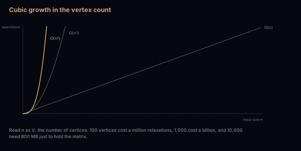
Time: O(V³), in every case. Count directly. The k loop runs V times, the i loop runs V times inside it, and the j loop runs V times inside that. The body is one read of dist[i][k], one of dist[k][j], one addition, one comparison and at most one write: all constant time. The total is exactly V³ relaxation attempts, which for the five-vertex graph above is 5³ = 125, matching the trace.
There is no best case and no worst case. The loops have no early exit and cannot have one, because a single cheap edge discovered on the final sweep can improve cells anywhere in the table. An already-complete matrix costs exactly as much as an empty one.
Space: O(V²). One matrix of V² numbers plus a fixed number of scalars; keeping next_hop doubles the constant, not the exponent. This bound, not the time bound, is usually what stops you: at V = 10,000 the distance matrix alone holds 100 million floats, around 800 MB before a single next-hop pointer.
Against V runs of Dijkstra. This is the comparison that matters, and the honest answer is "it depends on density". Dijkstra with a binary heap costs O((V + E) log V) from one source, so all V sources cost O(V·E·log V) once E is at least V. Set that against V³:
| Graph | E | V runs of Dijkstra | Floyd-Warshall |
|---|---|---|---|
| Sparse, V = 1,000 | 3,000 | ~30 million | 1 billion |
| 10% dense, V = 1,000 | 100,000 | ~1 billion | 1 billion |
| Complete, V = 1,000 | 1,000,000 | ~10 billion | 1 billion |
The crossover sits where V·E·log V equals V³, which is where E is about V² / log V, roughly a tenth of all possible edges on a 1,000-vertex graph. Below that, repeated Dijkstra wins, and on genuinely sparse graphs it wins by orders of magnitude. Above it, Floyd-Warshall wins by more than the formulas suggest: its inner loop is a contiguous scan of two matrix rows with a perfectly predictable branch, while Dijkstra's is heap operations and pointer chasing.
Johnson's algorithm is the third option. One Bellman-Ford pass reweights the graph so every edge becomes non-negative, then Dijkstra runs from each source, giving O(V² log V + V·E) with a Fibonacci heap — or O(V·E·log V) with the binary heap above — and negative edges still allowed. On a sparse graph with negative weights it beats Floyd-Warshall comfortably, at the cost of several times more code.
When to use it, and when not to
Use it when V is small and you genuinely need every pair. A few hundred vertices is the comfortable zone: 500 vertices is 125 million relaxations, a fraction of a second in C and around twenty seconds in pure Python. If your graph fits and you want a lookup table you can query in O(1) forever after, this is the simplest correct thing you can write.
Use it when the graph is dense. Once most vertex pairs have an edge, E approaches V² and V runs of Dijkstra cost about V³ log V, so the triple loop is doing strictly less work, with a far better constant factor on top.
Use it when weights can be negative and V is small. Dijkstra is simply incorrect there, and Floyd-Warshall handles it with no extra code plus free negative-cycle detection.
Do not use it when the graph is sparse. A road network, a social graph or a dependency graph has far fewer than V² edges. Run Dijkstra once per source you actually care about, or use Johnson's algorithm if you truly need all pairs.
Do not use it when V is in the thousands. At V = 5,000 you are looking at 125 billion relaxations and a 200 MB matrix. Road routing at national scale uses contraction hierarchies or A* with landmarks, not an all-pairs table.
Do not use it when you only need one source. Computing V² answers to get V of them wastes a factor of V. Use BFS for unweighted graphs, Dijkstra for non-negative weights, Bellman-Ford for negative ones.
Where it shows up in the real world
Library implementations. SciPy ships scipy.sparse.csgraph.floyd_warshall, NetworkX ships networkx.floyd_warshall_predecessor_and_distance, and the Boost Graph Library ships floyd_warshall_all_pairs_shortest_paths. Python has no standard-library graph module at all, so at work SciPy is what you reach for rather than the loops above.
Chemistry software. A molecule is a graph with tens of atoms, so V³ is trivially cheap, and the all-pairs topological distance matrix is the starting point for classic molecular descriptors such as the Wiener index.
Converting automata to regular expressions. Kleene's algorithm eliminates the states of a finite automaton one at a time, tracking which strings get from state i to state j using only states up to k in between. That is the identical recurrence, with concatenation in place of addition and alternation in place of minimum.
Precomputed distance tables. When a navigation graph is a few hundred waypoints and never changes, computing the full table once at load time turns every later distance query into an array lookup. This is a standard trick for coarse region-level pathfinding in games, with a finer local search layered on top.
Bottleneck and reliability variants. Swap the operations again and the same loops answer different questions. Maximum over minimums gives the widest path: the route whose narrowest link is as wide as possible, which is the bandwidth question. Maximum over products gives the most reliable path when each edge has an independent success probability.
Common mistakes
Putting k in the wrong loop. This is the one. Here is the wrong version run on the graph from the walkthrough, printed against the correct answers.
def floyd_warshall_wrong(dist: list[list[float]]) -> list[list[float]]:
    """The classic bug: k as the innermost loop instead of the outermost."""
    n = len(dist)
    for i in range(n):
        for j in range(n):
            for k in range(n):
                through_k = dist[i][k] + dist[k][j]
                if through_k < dist[i][j]:
                    dist[i][j] = through_k
    return dist


correct = floyd_warshall(build_matrix(5, EDGES))
broken = floyd_warshall_wrong(build_matrix(5, EDGES))
print("pair      correct   i,j,k order")
for i in range(5):
    for j in range(5):
        if correct[i][j] != broken[i][j]:
            print(f"{NAMES[i]} to {NAMES[j]} {cell(correct[i][j]):>9}"
f"{cell(broken[i][j]):>13}")pair correct i,j,k order
B to A 10 .
B to C 12 .
C to A 11 12Twenty-two of the twenty-five cells are right, which is exactly what makes this bug dangerous. The three that are wrong are wrong in both possible ways: C to A comes back as 12 instead of 11, an overestimate along a real but suboptimal route, while B to A and B to C come back as unreachable when routes of cost 10 and 12 exist. A test that only checks a handful of pairs will pass.
Using a large integer as infinity. Writing INF = 999999 and then computing INF + INF gives 1,999,998, which is less than some legitimate comparison and quietly corrupts a cell. Worse, in C or Java it overflows to a negative number and the corruption becomes spectacular. float("inf") has neither problem. If you must use an integer sentinel, guard the relaxation with a check that both operands are finite.
Building the matrix with [[INF] * n] * n. The outer * n copies the reference to one row, so all n rows are the same list and writing one cell writes an entire column. Use a comprehension: [[INF] * n for _ in range(n)].
Forgetting to zero the diagonal. This one fails more quietly than people expect. Every off-diagonal cell still comes out correct, because the body only ever reads dist[i][k] and dist[k][j] and a route from i to j never needs the price of standing still. What breaks is the diagonal itself: leave dist[i][i] at infinity and it fills with the cheapest cycle through i instead of 0, on the five-vertex graph above every diagonal entry ends up as 13, the lap A to C to B to D to E to A. Any code that reads dist[i][i] as a distance then gets 13 where the answer is 0.
Trusting the numbers when the diagonal is negative. Once a negative cycle exists, the off-diagonal entries are arbitrary and route reconstruction can loop forever, because the next-hop pointers may form a cycle. Check dist[v][v] < 0 for every v before reading anything else.
Treating an undirected graph as directed. An undirected edge is two entries, dist[i][j] and dist[j][i]. Set only one and the matrix describes a one-way street system.
Practice
- Add a
vertex_countof 6 to the example graph with a vertex F that nothing points to and that points to nothing, and confirm its row and column stay infinite apart fromdist[F][F]. - Modify
floyd_warshallto raise aValueErrornaming the first vertex it finds with a negative diagonal entry, and test it on the three-vertex negative cycle above. - Write the widest-path variant: replace the relaxation with maximum of minimums, so
dist[i][j]becomes the largest possible bottleneck capacity between i and j. - Compute the graph's diameter — the largest finite entry in the completed matrix — and the vertex whose greatest distance to anywhere is smallest, which is its centre.
- Implement the bit-set transitive closure: store each row as a Python integer, and replace the inner j loop with
reach[i] |= reach[k]. Confirm it agrees with the boolean version on a 200-vertex random graph.
Summary
Floyd-Warshall is a dynamic program wearing a very plain disguise. Layer k of the DP is "shortest routes allowed to pass through the first k vertices", each layer is built from the one below it in a single sweep of the matrix, and the loop nesting is what enforces that ordering. Get k on the outside and you get every shortest path in the graph in about ten lines. Get it anywhere else and you get a table that looks right and is not.
| Difficulty | Hard |
| Time (all cases) | O(V³) — three nested loops of V, constant work inside, no early exit |
| Space | O(V²) — one distance matrix; a second one for route reconstruction |
| Answers | All V² vertex pairs in one run |
| Handles negative weights | Yes — unlike Dijkstra |
| Detects negative cycles | Yes — a negative entry on the diagonal |
| Reconstructs paths | Yes — with an O(V²) next-hop matrix |
| Data structure | Adjacency matrix, a list of lists of floats |
| Use it when | V is a few hundred, the graph is dense, or you need every pair |
| Avoid it when | The graph is sparse, V is in the thousands, or you need one source |
| Real-world use | SciPy, NetworkX and Boost implementations; molecular distance matrices; Kleene's algorithm |
| Python equivalent | scipy.sparse.csgraph.floyd_warshall — no standard-library version exists |
Learn it for the recurrence rather than the code. The trick of enlarging a permitted set one element at a time, and letting the outer loop carry that enlargement, shows up all over dynamic programming. It is the same move as the item index in knapsack and the prefix length in edit distance.
Keep reading
- Dijkstra's Algorithm — the single-source alternative, and the one to run V times when your graph is sparse.
- Bellman-Ford — single-source shortest paths with negative edges, and the reweighting step inside Johnson's algorithm.
- Dynamic Programming Explained — the general shape of the layer-by-layer argument used above.
- Graphs in Python — adjacency matrices versus adjacency lists, and why density decides everything here.
- Breadth-First Search — shortest paths when every edge costs the same, in O(V + E) instead of O(V³).


