Roads between towns, friendships, imports between Python modules, links between web pages, legal moves in a sliding puzzle. Those five have nothing in common except their shape: a set of things, and a set of connections between pairs of them. That shape is a graph, and it is the most general structure in this series: a linked list is a graph, a tree is a graph, a grid is a graph, each with extra rules bolted on.
The payoff for noticing is large. Once a problem is written as vertices and edges, a shelf of ready-made algorithms opens up: shortest route, cheapest route, is-everything-reachable, what-order-can-these-tasks-run-in, is-there-a-cycle. You do not invent anything. You translate.
First you have to store the graph, and there are three ways to do it. They differ by orders of magnitude in memory and in lookup cost, and the choice silently fixes the running time of everything built on top: the same traversal is O(V + E) with one representation and O(V²) with another. Here is the vocabulary, all three representations on one worked example, and a small Graph class you can reuse.
The idea
A graph is two things.
Vertices (also called nodes) are the objects: towns, people, web pages, tasks, board positions.
Edges are the connections. An edge joins exactly two vertices and says "these two are directly related".
That is the whole definition. Everything else is vocabulary for describing a flavour of graph, or machinery for storing one.
Here is the graph this post uses throughout: five towns, A to E, joined by six roads: A–B, A–C, B–C, B–D, C–D and D–E.
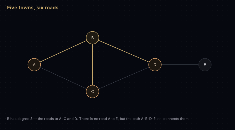
Three properties of that picture are what make graphs harder than the structures before them:
- There is no root and no order. A tree has a top; a list has a front. A graph has neither, so "the third vertex" means nothing and any vertex starts a traversal as well as any other.
- A vertex can have any number of edges, including zero. E has one, B has three, and an isolated town with no roads is still a valid vertex.
- Related does not mean adjacent. No road joins A and E, yet you can still drive A to B to D to E. That indirect reachability is what almost every graph algorithm is about.
The words you need
Graph vocabulary is small, and every term below reappears in the rest of the series.
Directed or undirected
An undirected edge works both ways, so it is just the unordered pair A–B. The road between those towns carries you in either direction; Facebook friendship is mutual by construction.
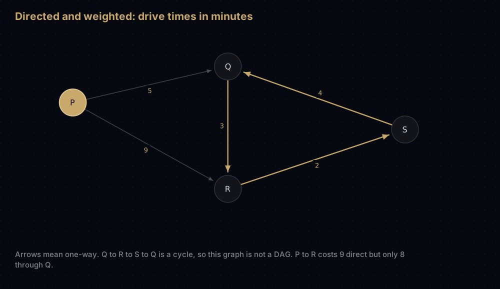
A directed edge points one way, and the graph is then a digraph. "compile must finish before link starts" is not the same statement as its reverse. Web links, Python imports, one-way streets and task dependencies are all directed, and storing P to Q does not store Q to P.
Weighted or unweighted
A weighted edge carries a number: kilometres, minutes, price, bandwidth. Unweighted is the special case where every edge costs the same, which is identical to every weight being 1.
This decides which algorithm you may use. On an unweighted graph the fewest-edges path is the shortest path, and breadth-first search finds it. Add weights and a two-edge detour can beat a one-edge road, so you need Dijkstra's algorithm instead.
Degree
The degree of a vertex is the number of edges touching it: B has degree 3, E has degree 1. Directed graphs split this into in-degree and out-degree.
A free sanity check hides here. Every edge has two ends, each adding 1 to some vertex's degree, so all degrees sum to exactly 2E. For the towns: 2 + 3 + 3 + 3 + 1 = 12, and 2 × 6 = 12. If yours do not sum to twice the edge count, the code adding edges has a bug.
Path, cycle, acyclic
A path is a sequence of vertices where each consecutive pair is joined by an edge. A–B–D–E is a path from A to E of length 3, because it uses three edges.
A cycle is a path that returns to its start without reusing an edge, such as A–B–C–A. A graph with no cycles is acyclic, and a directed acyclic graph is a DAG: the most useful special case there is. Git history, package dependencies and spreadsheet formulas are all DAGs. Topological sort exists only for DAGs, because a cycle admits no valid ordering.
Connected
A graph is connected when every vertex is reachable from every other. The towns graph is. Delete the road D–E and it is not, because E becomes its own component. Real graphs are often disconnected, which is why traversal code loops over all vertices instead of assuming one start point reaches everything.
Simple, dense, sparse
A simple graph has no self-loops and no repeated edge between the same pair. Assume simple unless told otherwise.
A simple undirected graph on V vertices has at most V(V − 1) / 2 edges, one per unordered pair, and that maximum is the yardstick for density. Dense means E is close to it, so E grows like V². Sparse means E is a small multiple of V.
Real graphs are overwhelmingly sparse, for a reason worth understanding rather than memorising: a road junction has three or four roads meeting at it whether the country has ten thousand junctions or ten million. Degree does not grow with the graph, so E stays proportional to V. Friendships, imports and outbound links behave the same way. Density is the one fact that decides your representation.
Three ways to store a graph
All three describe the same five towns and six roads. They differ only in what they make cheap.
Adjacency list
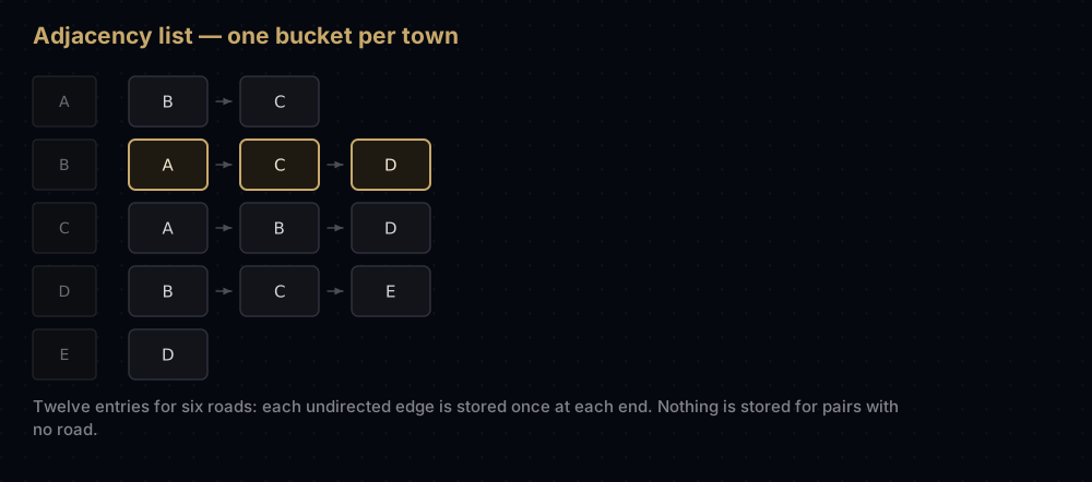
For each vertex, store the list of its neighbours. In Python that is a dictionary whose keys are vertices and whose values are lists.
A: [B, C]
B: [A, C, D]
C: [A, B, D]
D: [B, C, E]
E: [D]
Six roads, twelve entries — each undirected edge appears once in each endpoint's list, the same 2E count as the degree sum. Nothing is stored for pairs that are not connected, and that is the point: A–E appears nowhere.
Adjacency matrix
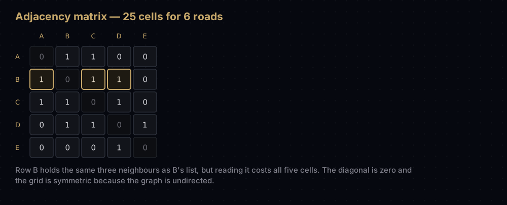
Number the vertices 0 to V − 1 and build a V by V grid. Cell (i, j) is 1 when there is an edge from i to j, and 0 when there is not.
   A B C D E
A  0 1 1 0 0
B  1 0 1 1 0
C  1 1 0 1 0
D  0 1 1 0 1
E  0 0 0 1 0
Every possible pair gets a cell whether or not the edge exists, so 25 numbers describe 6 roads. Two things fall straight out of the picture: the diagonal is all zeros because no town has a road to itself, and the grid is symmetric because the graph is undirected — cells (B, D) and (D, B) always agree. For a directed graph that symmetry disappears, and the asymmetry is the representation showing you the arrows.
Edge list
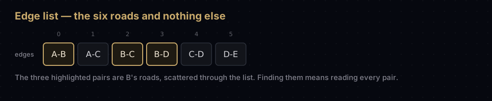
Just store the edges, as a flat list of pairs.
(A, B) (A, C) (B, C) (B, D) (C, D) (D, E)This is the smallest of the three and the least useful. It answers "what are all the edges?" perfectly and every other question badly: finding B's neighbours means reading all six pairs, or all million on a graph with a million edges. It cannot represent an isolated vertex at all: a town with no roads simply does not appear.
It survives because two algorithms genuinely want edges in bulk. Kruskal's minimum spanning tree sorts every edge by weight and consumes them in order; Bellman-Ford relaxes every edge, V − 1 times over. Both are clumsier written any other way.
The code
The adjacency list is the default, so it gets the real class. Two methods do the work: add_edge puts a connection in, neighbours takes one vertex out.
class Graph:
    """A graph stored as an adjacency list: one dict key per vertex, holding
    that vertex's neighbours.

    Undirected by default, so add_edge records the connection at both ends.
    Pass directed=True for one-way edges such as task dependencies or links.
    """

    def __init__(self, directed: bool = False) -> None:
        self.directed = directed
        self.adjacency: dict[str, list[str]] = {}

    def add_vertex(self, vertex: str) -> None:
        # setdefault, not assignment: re-adding an existing vertex must not
        # wipe the neighbours it already has.
        self.adjacency.setdefault(vertex, [])

    def add_edge(self, source: str, target: str) -> None:
        self.add_vertex(source)
        self.add_vertex(target)
        self.adjacency[source].append(target)
        if not self.directed:
            self.adjacency[target].append(source)

    def neighbours(self, vertex: str) -> list[str]:
        """Everything reachable from `vertex` in exactly one step."""
        return self.adjacency.get(vertex, [])

    def vertices(self) -> list[str]:
        return list(self.adjacency)

    def degree(self, vertex: str) -> int:
        return len(self.neighbours(vertex))

    def edges(self) -> list[tuple[str, str]]:
        """Every edge once. An undirected edge is stored twice, so keep only
        the copy whose endpoints are already in label order.
        """
        found: list[tuple[str, str]] = []
        for source, targets in self.adjacency.items():
            for target in targets:
                if self.directed or source <= target:
                    found.append((source, target))
        return found


towns = Graph()
for one, other in [("A", "B"), ("A", "C"), ("B", "C"),
                   ("B", "D"), ("C", "D"), ("D", "E")]:
    towns.add_edge(one, other)

print("vertices:       ", towns.vertices())
print("neighbours of B:", towns.neighbours("B"))
print("neighbours of E:", towns.neighbours("E"))
print("degree of B:    ", towns.degree("B"))
print("edges:          ", towns.edges())
print("V =", len(towns.vertices()), " E =", len(towns.edges()))vertices: ['A', 'B', 'C', 'D', 'E']
neighbours of B: ['A', 'C', 'D']
neighbours of E: ['D']
degree of B: 3
edges: [('A', 'B'), ('A', 'C'), ('B', 'C'), ('B', 'D'), ('C', 'D'), ('D', 'E')]
V = 5 E = 6The same class handles directed graphs by skipping one line. Here is a build pipeline where parsing precedes compiling, and compiling precedes both linking and testing:
builds = Graph(directed=True)
for before, after in [("parse", "compile"), ("compile", "link"), ("compile", "test")]:
    builds.add_edge(before, after)

print("compile unlocks:", builds.neighbours("compile"))
print("link unlocks: ", builds.neighbours("link"))compile unlocks: ['link', 'test']
link unlocks: []link has an empty neighbour list even though an edge touches it, because an incoming arrow says nothing about where you can go next. That asymmetry is the whole difference between the two modes.
The matrix version needs the full set of labels up front, since you cannot size a V by V grid before you know V.
class MatrixGraph:
    """The same graph as a V by V grid of 0s and 1s.

    The label-to-row mapping is built once and kept, so an edge test is two
    dict lookups and one indexed read -- constant time, whatever V is.
    """

    def __init__(self, labels: list[str], directed: bool = False) -> None:
        self.labels = list(labels)
        self.position = {label: index for index, label in enumerate(self.labels)}
        self.directed = directed
        size = len(self.labels)
        self.matrix = [[0] * size for _ in range(size)]

    def add_edge(self, source: str, target: str) -> None:
        self.matrix[self.position[source]][self.position[target]] = 1
        if not self.directed:
            self.matrix[self.position[target]][self.position[source]] = 1

    def has_edge(self, source: str, target: str) -> bool:
        return self.matrix[self.position[source]][self.position[target]] == 1

    def neighbours(self, vertex: str) -> list[str]:
        """Reading a row means touching all V cells, even for a vertex with
        one neighbour. This is the matrix's real cost.
        """
        row = self.matrix[self.position[vertex]]
        return [self.labels[index] for index, value in enumerate(row) if value]


grid_of_towns = MatrixGraph(sorted(towns.vertices()))
for source, target in towns.edges():
    grid_of_towns.add_edge(source, target)

print("   " + " ".join(grid_of_towns.labels))
for label, row in zip(grid_of_towns.labels, grid_of_towns.matrix):
    print(f"{label}  " + " ".join(str(value) for value in row))

print("ones in the matrix:", sum(sum(row) for row in grid_of_towns.matrix))
print("neighbours of B:   ", grid_of_towns.neighbours("B"))
print("edge B-D?", grid_of_towns.has_edge("B", "D"), " edge A-E?", grid_of_towns.has_edge("A", "E")) A B C D E
A 0 1 1 0 0
B 1 0 1 1 0
C 1 1 0 1 0
D 0 1 1 0 1
E 0 0 0 1 0
ones in the matrix: 12
neighbours of B: ['A', 'C', 'D']
edge B-D? True edge A-E? FalseTwelve ones, which is 2E again. Both structures agree that B's neighbours are A, C and D; they paid very different prices to say so.
Finally, weights. Store the cost alongside the endpoint instead of the endpoint alone, and the algorithms that walk outward from a vertex — Dijkstra above all — accept this shape directly.
class WeightedGraph:
    """An adjacency list whose entries carry the edge cost as well as the
    endpoint. Dijkstra and anything else that expands one vertex at a time
    reads this shape directly.
    """

    def __init__(self, directed: bool = False) -> None:
        self.directed = directed
        self.adjacency: dict[str, list[tuple[str, float]]] = {}

    def add_edge(self, source: str, target: str, weight: float) -> None:
        self.adjacency.setdefault(source, []).append((target, weight))
        self.adjacency.setdefault(target, [])
        if not self.directed:
            self.adjacency[target].append((source, weight))

    def neighbours(self, vertex: str) -> list[tuple[str, float]]:
        return self.adjacency.get(vertex, [])


roads = WeightedGraph(directed=True)
for source, target, minutes in [("P", "Q", 5), ("P", "R", 9),
                                ("Q", "R", 3), ("R", "S", 2), ("S", "Q", 4)]:
    roads.add_edge(source, target, minutes)

print("leaving P:", roads.neighbours("P"))
print(f"P to R: the direct road costs 9, but P -> Q -> R costs {5 + 3}")leaving P: [('Q', 5), ('R', 9)]
P to R: the direct road costs 9, but P -> Q -> R costs 8That last line is why weighted graphs get their own algorithms. The direct road from P to R is a single edge and still the slower option, so "fewest edges" and "shortest" become different questions the moment weights exist.
How the code maps to the idea
add_edge writes twice when the graph is undirected. One fact stored in two places, because "who are B's neighbours?" must be answerable by looking only at B. That duplication is deliberate, it is where the 2E in the space bound comes from, and forgetting it is the most common graph bug there is.
add_vertex uses setdefault, not assignment. Writing self.adjacency[vertex] = [] would erase a vertex's neighbours every time another edge touched it. setdefault inserts an empty list only for a genuinely new key, which also lets an isolated vertex exist.
neighbours uses .get(vertex, []) rather than indexing. Asking about a vertex that is not in the graph returns an empty list instead of raising KeyError, and a read never modifies the graph. That is exactly the trap collections.defaultdict(list) sets: with a defaultdict, graph[vertex] inserts a new empty key as a side effect of looking.
edges deduplicates with source <= target. Every undirected edge is stored at both endpoints, so a naive walk reports each one twice; keeping only the copy already in label order gives exactly one of each. One blind spot: a self-loop A–A satisfies A <= A from both directions and is emitted twice. Simple graphs have none, but if yours might, track seen pairs in a set instead.
MatrixGraph builds position once, in the constructor. This is what makes the O(1) edge test honest. If has_edge rebuilt the label-to-index mapping per call it would be doing O(V) work each time, and the matrix's one advantage would evaporate.
MatrixGraph.neighbours scans a whole row. Five cells to find three neighbours here; a million cells to find three neighbours on a graph with a million vertices. The matrix cannot skip the zeros.
Complexity
Let V be the number of vertices and E the number of edges.
Adjacency list space: O(V + E). One dictionary key per vertex gives V, and each undirected edge contributes one list entry at each of its two endpoints, giving 2E. Total V + 2E; constants drop, so O(V + E). Both terms matter — a graph of a million vertices with no edges still costs a million keys.
Adjacency matrix space: O(V²). V rows of V cells, and every cell exists whether or not its edge does. The edge count does not appear in the bound at all: 1,000 vertices means 1,000,000 cells whether the graph has 3 edges or 400,000.
Edge list space: O(E). One pair per edge and nothing else, which is why isolated vertices vanish.
Now the queries. Here is one lookup run against each representation, counting what it really had to read:
def list_lookup_cost(graph: Graph, source: str, target: str) -> int:
    """Neighbour entries read before the adjacency list can answer."""
    read = 0
    for neighbour in graph.neighbours(source):
        read += 1
        if neighbour == target:
            break
    return read


def edge_list_lookup_cost(pairs: list[tuple[str, str]], source: str, target: str) -> int:
    """Pairs read before a flat edge list can answer."""
    read = 0
    for one, other in pairs:
        read += 1
        if (one, other) in ((source, target), (target, source)):
            break
    return read


pairs = towns.edges()
for source, target in [("B", "D"), ("A", "E")]:
    print(f"is there an edge {source}-{target}? "
          f"list reads {list_lookup_cost(towns, source, target)}, "
          f"matrix reads 1, "
f"edge list reads {edge_list_lookup_cost(pairs, source, target)}")is there an edge B-D? list reads 3, matrix reads 1, edge list reads 4
is there an edge A-E? list reads 2, matrix reads 1, edge list reads 6The list read B's three neighbours; the matrix read one cell. The gap looks trivial at V = 5 and is not trivial at V = 5,000,000, which is the trade the table below prices.
| Operation | Adjacency list | Adjacency matrix | Edge list |
|---|---|---|---|
| Space | O(V + E) | O(V²) | O(E) |
| Add an edge | O(1) | O(1) | O(1) |
| Is there an edge u–v? | O(degree of u) | O(1) | O(E) |
| List u's neighbours | O(degree of u) | O(V) | O(E) |
| Remove an edge | O(degree of u + degree of v) | O(1) | O(E) |
| Visit every edge | O(V + E) | O(V²) | O(E) |
| Add a vertex | O(1) | O(V²) — regrow the grid | Not possible — no isolated vertices |
Two rows there decide almost every real choice.
"Is there an edge?" is the matrix's win, and a genuine one: two dictionary lookups to turn labels into indices plus one indexed read into a list of lists, none of which grows with V. The indexed read is constant time outright; the dictionary lookups are constant on average, which is the assumption sitting under every dict cost in this post. The adjacency list must scan one neighbour list, holding degree-of-u entries and in the worst case V − 1 of them.
"Visit every edge" is the list's win, and it is far bigger. Traversals such as breadth-first search and depth-first search visit each vertex once and, at each, walk that vertex's neighbours. All degrees together sum to 2E, so the total is V + 2E. That is, O(V + E). Run the identical traversal on a matrix and each visit reads a full row of V cells: V vertices times V cells is O(V²), and it stays O(V²) on a graph with three edges. On a road network with 24 million junctions that is the difference between finishing and never finishing.
The same story shows up in memory:
print(f"{'vertices':<12} {'edges':<12} {'matrix cells':<20} {'list entries'}")
for vertex_count, edge_count in [(1_000, 5_000), (1_000, 400_000), (24_000_000, 29_000_000)]:
    print(f"{vertex_count:<12,} {edge_count:<12,} "
f"{vertex_count * vertex_count:<20,} {vertex_count + 2 * edge_count:,}")vertices edges matrix cells list entries
1,000 5,000 1,000,000 11,000
1,000 400,000 1,000,000 801,000
24,000,000 29,000,000 576,000,000,000,000 82,000,000Row one is sparse: the matrix costs 90 times more memory for the same information. Row two is the same 1,000 vertices packed with 400,000 edges — 80% of the 499,500 possible — and now the two are within a small factor, the matrix's flat integers competing well against the list's dictionary and list overhead. Row three is the standard DIMACS benchmark road network of the continental United States: roughly 24 million junctions and 29 million road segments, which that dataset stores as 58 million directed arcs, one per direction. The list needs about 82 million entries. The matrix needs 576 trillion cells, over 70 terabytes at one bit per cell. No machine makes that the right answer.
Which representation to use
Use an adjacency list by default. It is right for sparse graphs, real-world graphs are almost always sparse, and it is optimal for the operation you perform most: listing a vertex's neighbours in time proportional to how many there are. You cannot enumerate k things in fewer than k steps, so it wastes nothing.
Use an adjacency matrix when the graph is dense, meaning E is a substantial fraction of V², or when V is small enough that V² is free and edge tests dominate. A few thousand vertices is a comfortable ceiling: V = 2,000 is 4 million cells, which is nothing; V = 200,000 is 40 billion cells, which is impossible. Floyd-Warshall is the clearest case. It is O(V³) anyway, so it only ever runs on small graphs, and it wants exactly the "cost from i to j" grid a matrix already is.
Use an edge list when your algorithm consumes edges in bulk and never asks about one vertex: Kruskal sorting edges by weight, Bellman-Ford relaxing all of them repeatedly, or simply reading a graph from a file, since input formats are nearly always lists of pairs. Convert to an adjacency list the moment you need a vertex's neighbours.
What Python gives you. There is no graph type in the standard library, and you do not need one: dict[str, list[str]] is the representation. The nearest thing to a built-in graph API is graphlib.TopologicalSorter (Python 3.9 and later), which takes a plain dictionary mapping each node to an iterable of its predecessors and orders a DAG for you. collections.defaultdict(list) saves the setdefault call if you respect the accidental-insert trap above.
Grids are graphs too
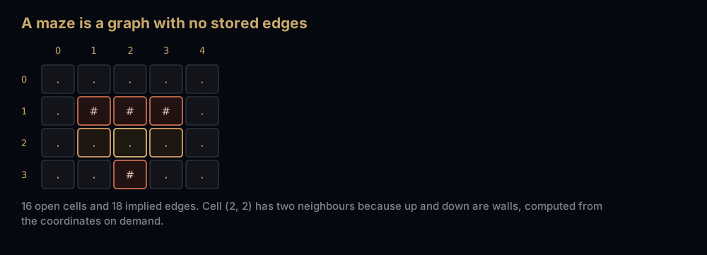
Not every graph needs storing. A maze, a chessboard, an image, a tile map — anything on a grid — is a graph whose edges are implied by the coordinates, so you compute neighbours on demand and store no edges at all. This is an implicit graph, and it is how nearly every pathfinding problem you meet is actually represented.
MAZE = [
    ".....",
    ".###.",
    ".....",
    "..#..",
]

STEPS = ((-1, 0), (1, 0), (0, -1), (0, 1))


def maze_neighbours(maze: list[str], cell: tuple[int, int]) -> list[tuple[int, int]]:
    """The open cells one step up, down, left or right.

    No edges are stored anywhere: the neighbours are recomputed from the
    coordinates every time they are asked for.
    """
    row, column = cell
    found: list[tuple[int, int]] = []
    for row_step, column_step in STEPS:
        next_row, next_column = row + row_step, column + column_step
        inside = 0 <= next_row < len(maze) and 0 <= next_column < len(maze[0])
        if inside and maze[next_row][next_column] != "#":
            found.append((next_row, next_column))
    return found


print("neighbours of (0, 0):", maze_neighbours(MAZE, (0, 0)))
print("neighbours of (2, 2):", maze_neighbours(MAZE, (2, 2)))

open_cells = [(row, column)
              for row in range(len(MAZE))
              for column in range(len(MAZE[0]))
              if MAZE[row][column] == "."]
implied = sum(len(maze_neighbours(MAZE, cell)) for cell in open_cells) // 2
print(f"the maze is a graph with {len(open_cells)} vertices and {implied} edges, "
f"none of them stored")neighbours of (0, 0): [(1, 0), (0, 1)]
neighbours of (2, 2): [(2, 1), (2, 3)]
the maze is a graph with 16 vertices and 18 edges, none of them storedCorner cell (0, 0) has two neighbours because two of its four steps fall off the board. Cell (2, 2) also has two, for a different reason: up and down are walls. Every graph algorithm in this series works unchanged here: swap graph.neighbours(vertex) for maze_neighbours(maze, cell) and BFS finds the shortest route through the maze.
Where it shows up in the real world
Git. A repository's history is a directed acyclic graph of commits, each storing pointers to its parents: an adjacency list of predecessors, exactly the shape graphlib.TopologicalSorter expects. git log --graph draws that structure.
Package managers and build systems. pip, npm, apt, Make and Bazel all resolve dependencies before doing anything, and what they want is a DAG, because a cycle admits no build order. They differ on how hard they insist: Bazel rejects a dependency cycle outright, while GNU Make prints a circular-dependency warning, drops the offending edge and builds anyway.
Routing engines. OpenStreetMap-based routers hold road networks as adjacency lists over tens of millions of junctions, for the memory reason computed above.
Compilers. Register allocators use both representations at once on the interference graph: a bit matrix answers "do these two values overlap?" in constant time, while adjacency lists let the colouring pass walk a node's neighbours without touching V cells. When both queries must be fast and V is bounded, paying for both structures is legitimate.
Social and link graphs. Facebook's TAO stores the social graph as objects and associations: an edge-centric layout that is an adjacency list sharded across machines. PageRank runs over the web link graph, which at billions of pages could only ever be sparse-encoded.
Common mistakes
Forgetting the reverse edge. Appending only to adjacency[source] in an undirected graph gives you a directed graph in disguise. It passes any test that walks edges in the insertion direction and fails the moment something searches the other way. Symptom: a path exists from A to E but not from E to A.
Letting defaultdict grow the graph. With collections.defaultdict(list), graph[vertex] inserts a new empty key when the vertex is missing, so one typo in a read-only lookup silently adds a phantom vertex and V drifts upward. Read with .get(vertex, []).
Mutating the list neighbours hands back. It is the live internal list, not a copy: a copy would cost a fresh allocation and a second O(degree) walk on every single lookup, which is a price a traversal pays at every vertex. So graph.neighbours("B").remove("A") really does delete half an edge, leaving A pointing at a B that no longer points back. Delete through a remove_edge method that fixes both ends.
Adding the same edge twice. The adjacency list stores the duplicate happily, so B appears in D's list twice and degree reports 4 where the graph has 3 roads. The matrix hides it, because setting a cell to 1 twice changes nothing. If duplicates are possible, check before appending or hold a set per vertex.
Reaching for the matrix because O(1) beats O(degree). Wrong comparison. The operation your code runs thousands of times is "give me this vertex's neighbours", where the matrix costs O(V) against the list's O(degree). Choose on density, not on the edge-test row.
Practice
- Add
remove_edge(source, target)toGraphso it deletes both stored copies when the graph is undirected, and one when it is directed. - Write
density(graph)returning E divided by V(V − 1) / 2, and print it for the towns graph and for a 100-vertex chain where each vertex joins only the next. - Write a function that rebuilds a
Graphfrom aMatrixGraph, and confirm the round trip preserves every edge of the towns example. - Give
Graphanin_degree(vertex)method for directed graphs, and use it to find every vertex in the build pipeline with no prerequisites. - Model a knight's legal moves on an 8 by 8 chessboard as an implicit graph (a
knight_neighbours(square)function, no stored edges), and check that a corner square has exactly two moves.
Summary
A graph is vertices and edges, and the only real decision at this stage is how to store them. Use a dictionary of lists unless you can point at a specific reason not to: it costs O(V + E) memory, hands you a vertex's neighbours in time proportional to how many there are, and makes traversal O(V + E) instead of O(V²). Keep the matrix for dense graphs and small V, keep the edge list for algorithms that eat edges in bulk, and remember that grids need no storage at all.
| Difficulty | Easy |
| Space, adjacency list | O(V + E) — one key per vertex, two entries per undirected edge |
| Space, adjacency matrix | O(V²) — every cell exists whether the edge does or not |
| Space, edge list | O(E) — cannot represent an isolated vertex |
| Edge test | O(degree) list, O(1) matrix, O(E) edge list |
| List a vertex's neighbours | O(degree) list, O(V) matrix, O(E) edge list |
| Full traversal, BFS or DFS | O(V + E) list, O(V²) matrix |
| Add a vertex | O(1) list, O(V²) matrix — the grid must be regrown |
| Default choice | Adjacency list, a dict of lists |
| Use a matrix when | The graph is dense, or V is a few thousand and edge tests dominate |
| Avoid a matrix when | V is large and E grows like V — V² memory bought for nothing |
| Real-world use | Git commit DAGs, build and package dependency graphs, road routing, compiler interference graphs |
| Python equivalent | dict[str, list[str]] or collections.defaultdict(list); graphlib.TopologicalSorter for DAGs |
Everything in the graph family from here assumes this adjacency-list shape and this vocabulary. The next step is to actually walk one.
Keep reading
- Breadth-First Search — the first thing to do with a graph, and shortest paths on unweighted edges for free.
- Depth-First Search — the other traversal, and the base for cycle detection and connected components.
- Topological Sort — what DAGs are for: ordering tasks so every dependency comes first.
- Dijkstra's Algorithm — shortest paths once edges carry weights and detours can win.
- Hash Tables — why the dictionary underneath the adjacency list gives average-case O(1) vertex lookup.


