
Depth-first search is the traversal that commits. Standing on a node with three unexplored neighbours, it picks the first one and goes, and keeps going, one neighbour deeper each time, until it reaches something with nowhere left to go. Only then does it back up one step and try the alternative it walked past. Breadth-first search does the opposite: it fans out level by level, finishing everything one step away before it looks at anything two steps away. Both visit every reachable node exactly once. They differ only in the order, and the order is the entire point.
DFS is worth learning properly because it is the engine underneath a surprising number of other algorithms. Topological sort is a DFS with the finish times written down. Cycle detection is a DFS that notices when it walks into a node it has not finished yet. Tarjan's articulation points, maze generation, sudoku solvers and the mark phase of a tracing garbage collector are all DFS with something bolted on. Learn the walk and you get all of them.
Two things trip people up, and this post spends most of its time on them. The first is that the iterative version with an explicit stack visits nodes in a different order from the recursive version, unless you do one specific thing. The second is that cycle detection in an undirected graph and cycle detection in a directed graph need genuinely different rules, and using the undirected rule on a directed graph reports cycles that are not there.
The idea
A graph is a set of nodes with connections (edges) between them. Depth-first search answers "which nodes can I reach from here, and in what order do I meet them" like this:
- Visit the node you are standing on. Write it down as visited.
- Look at its neighbours in turn. For the first one you have not visited, go there and repeat from step 1.
- When a node has no unvisited neighbours left, back up to whoever sent you here and continue their list of neighbours.
- Stop when you back up out of the node you started from.
The visited set is not an optimisation. Without it, the very first cycle in the graph sends you round it forever. Every DFS keeps one.
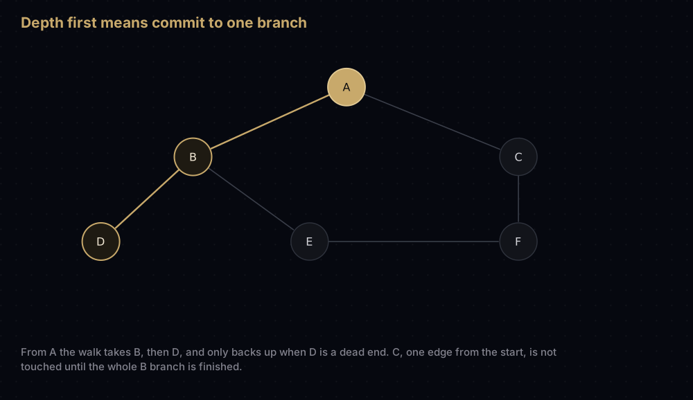
Notice what step 3 implies: the algorithm has to remember the way back. That memory is a stack: the nodes on your current path, most recent on top. Either you build it yourself in a list, or you let recursion build it out of function call frames. Same algorithm; the second version just hides the stack.
The graph in the diagram is the one used for the rest of this post. Six nodes, six undirected edges:
A — B      B — D      C — F
A — C      B — E      E — F
As adjacency lists, with each node's neighbours in alphabetical order:
A: B, C
B: A, D, E
C: A, F
D: B
E: B, F
F: C, E
Each undirected edge shows up twice, once from each end: A — B puts B in A's list and A in B's. That doubling matters later.
Watching it work
Start at A and follow the rules literally. Indentation is depth.
enter A               path: A
  enter B             path: A B          (A's first neighbour)
    A is visited, skip
    enter D           path: A B D
      B is visited, skip
    leave D                              D is finished first
    enter E           path: A B E
      B is visited, skip
      enter F         path: A B E F
        enter C       path: A B E F C
          A is visited, F is visited
        leave C
        E is visited, skip
      leave F
    leave E
  leave B
  C is visited, skip                     A's second neighbour, already done
leave A
The visit order is A, B, D, E, F, C.
Look at what happened to C. It is a direct neighbour of A — one edge away — and it is the last node visited, reached the long way round through B, E and F. That is depth-first behaviour in one observation. Distance from the start has nothing to do with visit order.
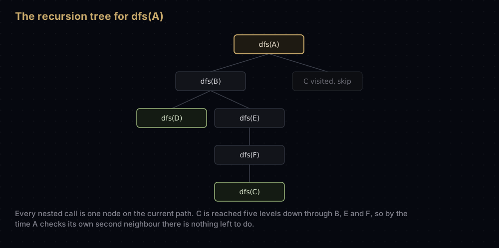
Now the same graph with an explicit stack. Push the start, then repeat: pop a node, and if it is new, visit it and push its unvisited neighbours.
pop   stack afterwards   visited so far
A     [B, C]             A
C     [B, F]             A C
F     [B, E]             A C F
E     [B, B]             A C F E
B     [B, D]             A C F E B
D     [B]                A C F E B D
B     []                 already visited — skipped
The visit order is A, C, F, E, B, D. Same graph, same starting node, same algorithm as usually described — different answer.
The reason is one line: A's neighbours are B, C, so you push B then C, and a stack hands back the last thing pushed. C comes out first. Recursion, by contrast, walks the neighbour list front to back. To make the stack agree with recursion, push the neighbour list backwards, so the front of the list ends up on top.
One more detail from that trace: B sits on the stack twice, pushed once by A and once by E, and the second copy is popped and thrown away. That is why the loop must re-check visited after popping.
The code
The recursive walk
Graph = dict[str, list[str]]

graph: Graph = {
    "A": ["B", "C"],
    "B": ["A", "D", "E"],
    "C": ["A", "F"],
    "D": ["B"],
    "E": ["B", "F"],
    "F": ["C", "E"],
}


def dfs_recursive(graph: Graph, start: str) -> list[str]:
    """Visit every node reachable from start, following one branch to its end
    before trying any alternative.

    The call stack does the bookkeeping: each pending `walk` frame is one node
    on the current path, waiting for its child to finish.
    """
    visited: set[str] = set()
    order: list[str] = []

    def walk(node: str) -> None:
        # Mark on entry, before recursing, or a cycle sends you round forever.
        visited.add(node)
        order.append(node)
        for neighbour in graph[node]:
            if neighbour not in visited:
                walk(neighbour)

    walk(start)
    return order


print(dfs_recursive(graph, "A"))['A', 'B', 'D', 'E', 'F', 'C']Five lines of logic. That is the whole algorithm, and it matches the indented trace above exactly.
The iterative walk, and why its order differs
def dfs_iterative(graph: Graph, start: str) -> list[str]:
    """The same traversal with an explicit stack instead of the call stack."""
    visited: set[str] = set()
    order: list[str] = []
    stack: list[str] = [start]

    while stack:
        node = stack.pop()
        # A node can sit on the stack in several places at once, pushed by
        # several neighbours, so re-check before doing any work.
        if node in visited:
            continue
        visited.add(node)
        order.append(node)
        for neighbour in graph[node]:
            if neighbour not in visited:
                stack.append(neighbour)

    return order


def dfs_iterative_matching(graph: Graph, start: str) -> list[str]:
    """Iterative DFS that reproduces the recursive visit order exactly."""
    visited: set[str] = set()
    order: list[str] = []
    stack: list[str] = [start]

    while stack:
        node = stack.pop()
        if node in visited:
            continue
        visited.add(node)
        order.append(node)
        # Pushed last is popped first, so push the neighbours backwards to
        # pop them forwards.
        for neighbour in reversed(graph[node]):
            if neighbour not in visited:
                stack.append(neighbour)

    return order


print(dfs_iterative(graph, "A"))
print(dfs_iterative_matching(graph, "A"))['A', 'C', 'F', 'E', 'B', 'D']
['A', 'B', 'D', 'E', 'F', 'C']The only difference between those two functions is reversed.
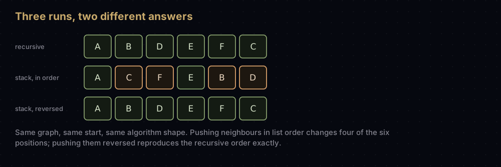
Both orders are legitimate: dfs_iterative produces exactly what recursion would produce if every adjacency list were reversed first. But when you are comparing against a textbook, a test fixture or a colleague's code, legitimate is not enough. Add reversed.
Numbering: pre-order and post-order
A DFS gives every node two useful numbers: when the walk entered it, and when the walk left it. Pre-order numbers count entries, post-order numbers count exits.
def dfs_numbers(graph: Graph, start: str) -> tuple[dict[str, int], dict[str, int]]:
    """Number each node when the walk enters it and again when it leaves."""
    pre: dict[str, int] = {}
    post: dict[str, int] = {}

    def walk(node: str) -> None:
        pre[node] = len(pre) + 1
        for neighbour in graph[node]:
            if neighbour not in pre:  # pre doubles as the visited set
                walk(neighbour)
        post[node] = len(post) + 1

    walk(start)
    return pre, post


pre_number, post_number = dfs_numbers(graph, "A")
for node in sorted(pre_number):
print(f"{node} pre {pre_number[node]} post {post_number[node]}")A pre 1 post 6
B pre 2 post 5
C pre 6 post 2
D pre 3 post 1
E pre 4 post 4
F pre 5 post 3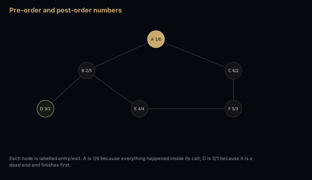
Read those numbers and the shape of the walk falls out. A is 1/6: entered first, left last, because everything else happened inside its call. D is 3/1: entered third, but the first to finish, because it is a dead end. Pre-order is the order you meet nodes going down. Post-order is the order they run out of work coming back up.
Post-order is the more useful of the two. A node's post number is assigned only after every node reachable from it has been visited. When the graph is acyclic that becomes something stronger: by the time a node gets its post number, everything reachable from it already has one, which is exactly the property a topological sort needs, and exactly the property that lets you compute anything about a subtree bottom-up. The stronger version genuinely needs acyclicity, and the numbers above show why: C finishes at post 2, but A — which C reaches in a single edge — does not finish until post 6.
Every component, not just one
dfs_recursive(graph, "A") finds what is reachable from A. A graph can be in several disconnected pieces, so to see all of it you restart the walk from every node you have not yet visited. Each restart discovers exactly one connected component.
def connected_components(graph: Graph) -> list[list[str]]:
    """Group the nodes so two nodes share a group exactly when a path joins them."""
    visited: set[str] = set()
    components: list[list[str]] = []

    for root in graph:
        if root in visited:
            continue
        component: list[str] = []
        stack = [root]
        while stack:
            node = stack.pop()
            if node in visited:
                continue
            visited.add(node)
            component.append(node)
            for neighbour in graph[node]:
                if neighbour not in visited:
                    stack.append(neighbour)
        components.append(sorted(component))

    return components


islands: Graph = {
    "A": ["B", "C"], "B": ["A", "D", "E"], "C": ["A", "F"],
    "D": ["B"], "E": ["B", "F"], "F": ["C", "E"],
    "G": ["H"], "H": ["G"],
    "I": [],
}
print(connected_components(islands))[['A', 'B', 'C', 'D', 'E', 'F'], ['G', 'H'], ['I']]The visited set is shared across restarts, which is what keeps the traversal linear: each node and each edge is touched once across the whole run, not once per component. The sorted(component) call is the one step that is not linear, and it buys nothing but a stable printed order: drop it and each component comes out in visit order instead.
Cycle detection in an undirected graph
In an undirected graph, every edge appears in both adjacency lists. So the moment you arrive at a node, one of its neighbours is guaranteed to be visited already: the node you just came from. That one edge is not a cycle. Any other edge to a visited node is.
from typing import Optional


def has_cycle_undirected(graph: Graph) -> bool:
    """True if any component of an undirected graph contains a cycle.

    Every undirected edge appears in both adjacency lists, so the edge you
    arrived on always points back at a visited node. That one edge is not a
    cycle; any other edge to a visited node is.
    """
    visited: set[str] = set()

    def walk(node: str, parent: Optional[str]) -> bool:
        visited.add(node)
        for neighbour in graph[node]:
            if neighbour not in visited:
                if walk(neighbour, node):
                    return True
            elif neighbour != parent:
                return True
        return False

    return any(walk(node, None) for node in graph if node not in visited)


tree: Graph = {
    "A": ["B", "C"], "B": ["A", "D", "E"], "C": ["A", "F"],
    "D": ["B"], "E": ["B"], "F": ["C"],
}
print(has_cycle_undirected(graph), has_cycle_undirected(tree))True FalseThe example graph has the cycle A — B — E — F — C — A; tree is the same graph with the E — F edge removed, and is now genuinely a tree. The walk finds the cycle at C, whose neighbour A is visited and is not C's parent F.
One honest caveat: comparing against the parent node breaks if the graph can have two parallel edges between the same pair of nodes, because the second copy also looks like "the edge I came in on". If that is possible in your data, pass the edge's identity down instead of the node's.
Cycle detection in a directed graph
Here is the trap. Take the undirected rule and point the edges:
Digraph = dict[str, list[str]]

diamond: Digraph = {"a": ["b", "c"], "b": ["d"], "c": ["d"], "d": []}
print(has_cycle_undirected(diamond))TrueThat is wrong. diamond is a → b → d and a → c → d: two paths converging on d, no cycle anywhere. The parent check fires because when the walk reaches c, its neighbour d is already visited and is not c's parent. Undirected, that would be a cycle. Directed, it is just a second route into a node that is already finished, and d leads nowhere, so nothing can loop back.
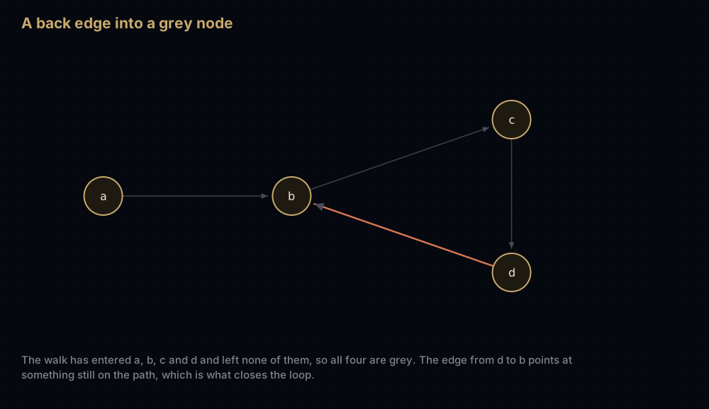
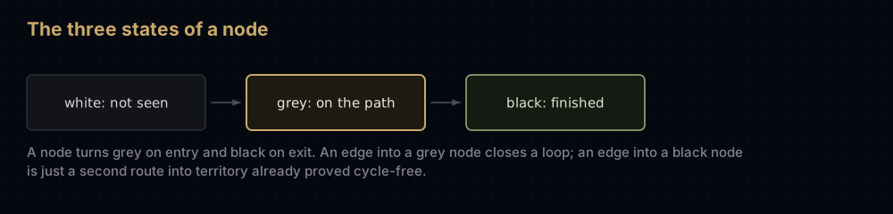
The correct rule tracks three states instead of two:
- white — not seen yet.
- grey — entered, not yet left. These are exactly the nodes on the current path, still sitting on the stack.
- black — left. Everything reachable from it has been fully explored.
An edge into a grey node is a back edge: it points at something still on the path below you, so following it closes a loop. An edge into a black node is harmless.
def has_cycle_directed(graph: Digraph) -> bool:
    """True if the directed graph contains a cycle.

    grey  = on the path currently being explored (still on the stack)
    black = fully explored, everything below it already checked

    An edge into a grey node closes a loop. An edge into a black node only
    re-enters a region that has already been proved cycle-free.
    """
    grey: set[str] = set()
    black: set[str] = set()

    def walk(node: str) -> bool:
        grey.add(node)
        for neighbour in graph[node]:
            if neighbour in grey:
                return True
            if neighbour not in black and walk(neighbour):
                return True
        grey.discard(node)  # leaving the node turns it from grey to black
        black.add(node)
        return False

    return any(walk(node) for node in graph if node not in black)


pipeline: Digraph = {"a": ["b"], "b": ["c"], "c": ["d"], "d": ["b"]}
print(has_cycle_directed(diamond), has_cycle_directed(pipeline))False Truediamond is now correctly acyclic, and pipeline — where d points back to b — is correctly cyclic. The grey set is just the recursion stack written down explicitly: you could instead ask "is this neighbour one of my callers", but a set answers that in O(1) rather than O(depth).
Reverse post-order is a topological order
A topological order lists every node before the nodes it points at: the order you would do a set of tasks in when the edges mean "must come first". DFS gives you one for free: reverse the post-order.
def topological_order(graph: Digraph) -> list[str]:
    """List every node before the nodes it points at. Requires a DAG."""
    visited: set[str] = set()
    finished: list[str] = []

    def walk(node: str) -> None:
        visited.add(node)
        for neighbour in graph[node]:
            if neighbour not in visited:
                walk(neighbour)
        # Appended only after every node reachable from here is done, so
        # `finished` is post-order.
        finished.append(node)

    for node in graph:
        if node not in visited:
            walk(node)

    return finished[::-1]


build: Digraph = {
    "app": ["ui", "core"],
    "ui": ["core"],
    "core": ["utils"],
    "utils": [],
}
print(topological_order(build))['app', 'ui', 'core', 'utils']The argument is short: a node is appended to finished only after everything it points at is already there, so in finished every node comes after its targets. Reverse it and every node comes before its targets. That is the definition.
Python ships a topological sort in the standard library, and it is the thing to reach for at work:
from graphlib import CycleError, TopologicalSorter

# graphlib takes the opposite direction: each key maps to what it depends on.
sorter = TopologicalSorter({"app": ["ui", "core"], "ui": ["core"], "core": ["utils"]})
print(list(sorter.static_order()))

try:
    TopologicalSorter({"b": ["d"], "c": ["b"], "d": ["c"]}).prepare()
except CycleError as error:
print("graphlib:", error.args[0])['utils', 'core', 'ui', 'app']
graphlib: nodes are in a cyclegraphlib.TopologicalSorter takes the edges the other way round — a key maps to what it depends on — and emits dependencies first, which is why its answer is the reverse of ours. It rejects cyclic input with CycleError. Internally it counts in-degrees rather than running a DFS; the topological sort post covers both methods.
How the code maps to the idea
visited.add(node) is the first statement in walk, not the last. Marking on entry is what makes the algorithm terminate on a cyclic graph. Move it after the loop and A → B → E → F → C → A runs forever.
The for loop over graph[node] is step 2, and the if neighbour not in visited guard is what stops you re-walking finished territory. Set membership is an average O(1) hash lookup, which is why using a list here instead of a set quietly turns the whole algorithm quadratic.
Returning from walk is step 3. There is no explicit "back up" code: when the loop ends the function returns, Python pops its frame, and control resumes in the caller's loop exactly where it left off. That is what popping your own stack does, which is why the two versions are one algorithm.
The parent argument exists only because undirected edges are stored twice. It is not a general DFS feature. In a directed graph there is no parent check at all, because an edge back to your caller genuinely is a cycle of length two.
grey.discard(node) before black.add(node) is the state transition, and getting it wrong is the classic bug. If you never remove a node from grey, the second time you reach a finished node it still looks like it is on the path, and you report a cycle in a perfectly good DAG.
Edge cases fall out for free. A lone node with no edges: walk runs once, the loop body never executes. An empty graph: connected_components loops over nothing and returns []. One case does not fall out: a node listed as a neighbour but missing as a key raises KeyError on graph[node], so use graph.get(node, []) or a collections.defaultdict(list) if your input might be ragged.
Python's recursion limit
CPython caps how deep the interpreter will recurse. The default is 1,000 frames, and a DFS on a long path burns one frame per node.
import sys

print(sys.getrecursionlimit())

long_path: Graph = {str(step): [str(step + 1)] for step in range(10_000)}
long_path["10000"] = []

try:
    dfs_recursive(long_path, "0")
    print("recursive walk finished")
except RecursionError:
    print("recursive walk: RecursionError")

print(len(dfs_iterative(long_path, "0")))1000
recursive walk: RecursionError
10001Ten thousand nodes in a line is not a large graph, and the recursive version cannot walk it. The iterative version does not care: its stack is a Python list on the heap, which grows until you run out of memory.
If you need the recursion, sys.setrecursionlimit raises the cap, but on its own it is not enough and it is dangerous: the limit exists to stop you overrunning the C stack, and overrunning that segfaults the process instead of raising an exception. The safe form is to ask for a bigger stack too, which you can only do for a new thread.
import threading


def dfs_deep(graph: Graph, start: str) -> list[str]:
    """Run the recursive walk on a thread with a stack big enough for it.

    Raising sys.setrecursionlimit on its own is not enough: the real ceiling
    is the C stack, and overrunning that segfaults instead of raising.
    """
    result: list[str] = []

    def target() -> None:
        sys.setrecursionlimit(30_000)
        result.extend(dfs_recursive(graph, start))

    threading.stack_size(64 * 1024 * 1024)
    worker = threading.Thread(target=target)
    worker.start()
    worker.join()
    return result


print(len(dfs_deep(long_path, "0")))10001That works, but it is a workaround. On graphs whose depth you do not control, write the iterative version instead.
Complexity
Time: O(V + E), where V is the number of nodes and E the number of edges. Both terms are earned, so count them separately.
The V term. walk adds its node to visited as its first action, and nothing calls walk on a node already in visited. So walk runs exactly once per reachable node: V calls, and each call does a constant amount of work outside its loop.
The E term. Inside a call the loop runs once per entry in graph[node], which is that node's degree. Sum the degrees over every node and you are counting every entry in the entire adjacency structure. In an undirected graph each edge is stored twice, so the sum is 2E. In a directed graph each edge is stored once, so it is E. Either way the total number of neighbour checks is proportional to E, and each check is one hash-set lookup.
V calls plus at most 2E neighbour checks: O(V + E). There is no best or worst case to speak of: every reachable node and every incident edge is examined once regardless of the input's shape. The one asterisk is visited: membership in a Python set is O(1) on average, not guaranteed, so O(V + E) is an average-case bound in the same sense that every hash-backed algorithm's is.
Why not simplify to O(E)? Because a graph can have far more nodes than edges. Ten thousand nodes and no edges at all still costs ten thousand steps, since the component loop must look at each one. The two terms measure different things and neither dominates in general.
One important dependency: this bound assumes an adjacency list, where graph[node] hands you exactly that node's neighbours. On an adjacency matrix finding the neighbours of one node means scanning a whole row of V entries, so DFS becomes O(V²): fine for a dense graph, wasteful for a sparse one.
Space: O(V), with one caveat. Three things use memory:
visitedholds at most one entry per node: O(V).- The recursive call stack holds one frame per node on the current path. Because
visitedprevents revisiting, that path is simple, so its length is at most V. O(V) — but the constant is a Python stack frame, which is far heavier than a list entry, and it is bounded by the recursion limit rather than by memory. - The explicit stack in
dfs_iterativeis the subtle one. A node gets pushed once for each edge that discovers it, so the stack can hold up to O(E) entries: genuinely more than O(V) on a dense graph. If that matters, push(node, iter(graph[node]))pairs and advance the top iterator one neighbour at a time instead of pushing all of them: that keeps a true depth-first order with at most V entries on the stack, mirroring the recursive version exactly.
When to use it, and when not to
Use DFS when the question is about reachability, structure or ordering: can I get from here to there, what are the components, is there a cycle, what order satisfies these dependencies, which nodes are single points of failure. Use it for exhaustive search too: every backtracking algorithm is a DFS over a tree of partial solutions.
Do not use it to find a shortest path. DFS finds a path, and on the example graph it reaches C — one edge from the start — after five other nodes. For fewest-edge paths on an unweighted graph use breadth-first search; with weighted edges use Dijkstra's algorithm.
| DFS | BFS | |
|---|---|---|
| Order | one branch to its end, then back up | everything 1 edge away, then 2, then 3 |
| Shortest path, unweighted | No | Yes |
| Peak memory | the current path — deep and narrow is cheap | the widest level — wide graphs are expensive |
| Natural form | recursion, or a list used as a stack | a collections.deque used as a queue |
| Gives you | post-order, topological order, cycles, bridges | distance layers, shortest paths |
The memory row is worth reading carefully, because it is weaker than it is usually sold as. It is decisive when the graph is implicit and there is no visited set: backtracking search over a tree of partial solutions, where DFS stores one branch and BFS would have to store a whole level. On an explicit graph both traversals already carry an O(V) visited set, so frontier versus path is a constant factor on top of that, and DFS's path is not automatically short: on a densely connected graph one branch can run through nearly every node before it dead-ends. Choose between them on the order you need, not on memory.
Also avoid recursive DFS on graphs whose depth you cannot bound. A 10,000-node chain is enough to kill it, as shown above.
Where it shows up in the real world
os.walk in Python's standard library is a depth-first traversal of a directory tree. With the default topdown=True it yields a directory's contents, then descends into the first subdirectory and everything beneath it before touching the second. It needs no visited set because a directory tree has no cycles, which is exactly why followlinks defaults to False, since symlinks can create one.
Build systems and package managers order work with a topological sort, which is the reverse post-order shown above. make updates a target's prerequisites before the target itself, recursively: a depth-first walk of the dependency graph.
Maze generation. The "recursive backtracker" is a randomised DFS on a grid: carve a passage to a random unvisited neighbour, keep going until stuck, back up and try another. Because it only carves into unvisited cells, the result is a spanning tree — exactly one path between any two cells — with the long winding corridors that DFS's commit-and-go-deep habit produces.
Puzzle solvers. Sudoku, N-queens and constraint solvers generally do DFS over a tree of partial assignments: place a value, recurse, back up when the partial solution becomes impossible. Pruning bad branches early is what makes this tractable.
Tarjan's algorithms. A single DFS that records each node's pre-order number and the lowest pre-order number reachable from its subtree finds all articulation points and bridges — the nodes and edges whose removal disconnects the graph — in one O(V + E) pass. The same low-link machinery finds strongly connected components.
Tracing garbage collectors. The mark phase walks the object graph from the roots (globals, stack frames, registers) and marks everything reachable; whatever stays unmarked is garbage. It is a traversal with a visited set, and it is normally written with an explicit mark stack rather than recursion, because object graphs get deep and a collector cannot afford to overflow the stack.
Common mistakes
No visited set. The single most common one. It works on trees, then hangs forever the first time the input has a cycle.
Marking visited when pushing instead of when popping. This caps the stack at V entries and still reaches everything, so it looks like an improvement. But a node's stack position is frozen at its first push, so a later, deeper discovery of it cannot pull it forward, and the visit order stops being depth-first. Fine for a pure reachability check; wrong for post-order numbering, topological sort or cycle detection.
Forgetting that a node can be on the stack twice. If you mark on pop, you must also check if node in visited: continue after popping, or a node gets visited more than once.
Using the undirected parent check on a directed graph. Demonstrated above: it reports a cycle in the acyclic diamond. Directed graphs need the grey/black distinction.
Never removing nodes from the recursion-stack set. Leaving a finished node in grey turns every re-entry into a false cycle report. grey.discard(node) on the way out is not optional.
Assuming the first path found is the shortest. DFS gives you a path. It is very often the long way round.
Expecting the iterative order to match the recursive order. It does not, unless you push the neighbour list reversed.
Practice
- Return the actual path from a start node to a target node, not just whether one exists, by carrying the current path down the recursion and copying it on success.
- Count the nodes in the largest connected component of an undirected graph.
- Given a grid of
1(land) and0(water), count the islands: run a DFS from every unvisited land cell over its four orthogonal neighbours. - Extend
has_cycle_directedso that it returns the nodes of the cycle it found, in order, rather than justTrue. - Rewrite
dfs_iterativeto push(node, iterator)pairs so that its order matchesdfs_recursiveand its stack never exceeds V entries.
Summary
Depth-first search is a walk with a stack and a visited set, and everything interesting comes from what you record along the way. Pre-order numbers give the order of discovery; post-order numbers give a topological sort and a bottom-up view of every subtree; the set of nodes currently on the stack gives cycle detection in a directed graph. The cost is one visit per node and one look per edge — O(V + E) — which is as good as anything that has to see the whole graph can be.
| Difficulty | Medium |
| Best case | O(V + E) — every reachable node and edge is examined once |
| Average case | O(V + E) |
| Worst case | O(V + E) — no input shape makes it worse |
| Space | O(V) — visited set plus a stack no deeper than the longest simple path; the naive explicit-stack form can reach O(V + E) |
| Detects cycles | Yes — parent check when undirected, grey set when directed |
| Shortest paths | No — use BFS on unweighted graphs, Dijkstra when weighted |
| Graph type | Directed or undirected; weights are ignored |
| Data structure | Adjacency list, a visited set, and a stack (explicit or the call stack) |
| Use it when | Reachability, components, cycles, topological order, backtracking search |
| Avoid it when | You need fewest-edge paths, or the graph is deeper than the recursion limit |
| Real-world use | os.walk, build dependency ordering, maze generation, Tarjan's articulation points, GC mark phase |
| Python equivalent | No stdlib DFS; graphlib.TopologicalSorter for DAG ordering, os.walk for directories |
Write the recursive version when the graph is small and you want the code to be obvious. Write the iterative version — with reversed — the moment the graph's depth is out of your control. And when the question is "which of these is closest", stop and reach for BFS instead.
Keep reading
- Breadth-First Search (BFS) — the other half of the pair, and the one that actually finds shortest paths.
- Graphs in Python — adjacency lists versus matrices, and why the choice changes DFS's complexity.
- Topological Sort — the DFS post-order trick and Kahn's in-degree algorithm, side by side.
- Recursion and Backtracking — the call stack model that makes recursive DFS obvious.
- Stacks in Python — the structure the iterative version is built on, explained from scratch.


