Dijkstra's algorithm is the one you reach for first, and it is genuinely faster. It also carries a precondition that is easy to forget: no edge may have a negative weight. The moment a weight can go below zero (a currency trade that gains you money, a rebate on a toll road) Dijkstra can return a wrong answer with complete confidence and no warning.
Bellman-Ford is what you use instead, and it is almost embarrassingly plain. Look at every edge in the graph and see whether it offers a cheaper route to the node it points at. Then do that V − 1 times, where V is the number of nodes. No priority queue, no visited set, no cleverness about which node to process next.
The interesting part is the number V − 1: why it is exactly right, and why one more round on top detects something Dijkstra cannot even express: a cycle of negative total weight, which means "shortest path" has no answer at all, because you can lap the cycle forever and keep getting cheaper. That extra round is what turns the algorithm into a currency arbitrage detector; the fact that a round needs nothing but each node's own neighbours is what put it inside the RIP routing protocol.
The idea
Everything rests on one operation, called relaxation. You keep an array distance holding your current best guess of the cost to reach each node from the source. Take any edge from tail to head with weight weight and ask one question: is distance[tail] + weight smaller than distance[head]? If it is, you have found a cheaper way to reach head (get to tail however you already know how, then take this one edge), so overwrite distance[head] with the smaller number.
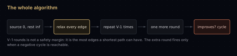
One addition, one comparison, one possible write. That is the algorithm's entire vocabulary. Bellman-Ford is then:
- Set
distance[source]to 0 and every other distance to infinity. - Relax every edge in the graph, in any fixed order. That is one round.
- Do V − 1 rounds.
No node is ever declared finished, and edges can be visited in whatever order they happen to sit in memory. That indifference is exactly what makes the algorithm robust against negative weights, and exactly what makes it slow.
Why not just use Dijkstra
Dijkstra settles nodes in increasing order of distance: it repeatedly takes the closest unsettled node, declares its distance final, and never looks at it again. That bet is safe when every weight is at least zero, because travelling further can only add cost. A negative edge breaks it.
Here is the smallest graph that shows the failure. Four nodes, with S -> A costing 1, S -> B costing 3, B -> A costing −5 and A -> T costing 1.
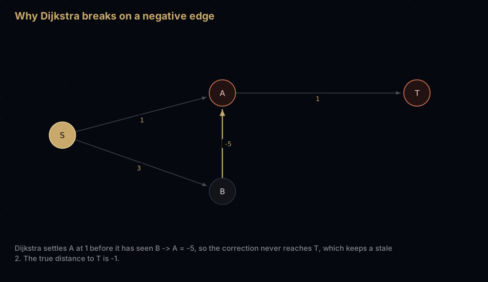
Dijkstra settles A at 1, because 1 is the smallest tentative distance on the table. It expands A and records T at 2. Only later does it reach B and relax B -> A down to −2, but A is settled, so that improvement never travels onward, and T keeps the stale 2. The true distance to T is −1.
Bellman-Ford has no settled set to be wrong about. When A drops to −2, the next round relaxes A -> T again and the correction propagates. Being willing to revisit everything, forever, is both the price and the point.
Why V − 1 rounds are enough
The loop bound looks arbitrary. It is not, and the argument is the most valuable thing in this post.
The invariant. After round k, for every node v, distance[v] is at most the weight of the cheapest walk from the source to v that uses k edges or fewer. ("Walk" rather than "path" because repeated nodes are allowed for now: that matters shortly.)
Base case, k = 0. Before any round runs, distance[source] is 0, the weight of the zero-edge walk that stays put, and every other distance is infinity. No other node is reachable in zero edges, so there is nothing for the claim to fail against.
Inductive step. Assume the invariant after round k − 1. Pick a node v and let P be a cheapest walk to v using at most k edges. If P has no edges then v is the source and its distance is already 0. Otherwise split P into a walk P' ending at some node u, followed by one edge from u to v of weight w.
P' uses at most k − 1 edges, and it must be a cheapest such walk to u: a cheaper one could be substituted to beat P, contradicting how P was chosen. So after round k − 1, distance[u] is at most weight(P').
Round k relaxes every edge, including the one from u to v. When it does, distance[u] is at most whatever it was after round k − 1, because distances only ever fall. So the relaxation leaves distance[v] at most distance[u] + w, which is at most weight(P') + w — exactly weight(P). Distances never rise, so the bound survives the rest of the round.
The other direction. Every value ever written is distance[tail] + weight for a real edge, so by the same induction every stored distance is the weight of a genuinely walkable route. distance[v] therefore never dips below the true shortest distance. Squeeze the two together: after round k, distance[v] sits between the true answer and the cheapest walk using at most k edges. As soon as some best walk fits inside k edges, the ends meet and the value is exact.
So how many edges can a shortest path need? Assume no negative cycle is reachable. Take any cheapest walk that visits a node twice and cut out the loop between the two visits. That loop is a cycle, its weight is not negative, so deleting it cannot make the walk more expensive, and it strictly removes edges. Repeat until no node repeats. What is left is a simple path, and a simple path through V nodes visits at most V of them, so it has at most V − 1 edges.
Feed that back into the invariant: after round V − 1 every distance is final. The bound is not a safety margin. It is precisely the longest a shortest path can possibly be.
And the extra round. Run one more round. If any edge still improves a distance, some route beats every route with at most V − 1 edges, so the best route needs V edges or more, so it repeats a node, so it contains a cycle, and cutting that cycle out would have cost nothing unless the cycle's own weight is negative. Conversely, if a reachable negative cycle exists, one more lap always lowers the total, so distances never stop falling and some edge is always relaxable. The extra round fires if and only if a negative cycle is reachable from the source. It is an exact test, not a heuristic.
Watching it work
Five nodes, six edges, one negative weight, source A: A -> B costs 5, A -> C costs 9, B -> C costs 3, C -> D costs −1, D -> E costs 2, B -> E costs 11.
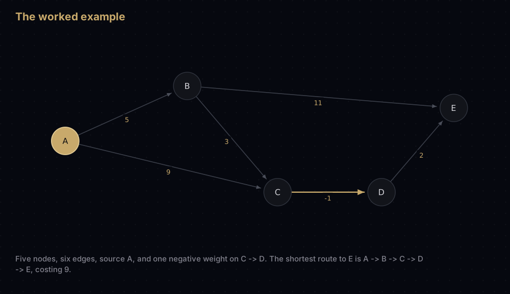
The edge list is deliberately stored back to front (D -> E, C -> D, B -> C, A -> B, A -> C, B -> E), which is the worst possible order and is what makes the round structure visible.
Round 1 walks the list top to bottom:
D -> E:distance[D]is still infinity, so this edge has nothing to offer. Skip.C -> D: infinity again. Skip.B -> C: infinity again. Skip.A -> B: 0 + 5 beats infinity, sodistance[B]becomes 5.A -> C: 0 + 9 beats infinity, sodistance[C]becomes 9.B -> E: 5 + 11 = 16 beats infinity, sodistance[E]becomes 16.
Half the edges did nothing, because they start from nodes the algorithm had not reached yet. That waste is the cost of not caring about order.
Round 2. C -> D gives 9 − 1 = 8, so distance[D] becomes 8. Then B -> C gives 5 + 3 = 8, beating the 9 the direct edge offered, so distance[C] becomes 8. Note the sequencing: C -> D used the stale 9, so D's new 8 is already wrong by one, and nothing later in this round fixes it.
Round 3. D -> E gives 8 + 2 = 10, beating 16. Then C -> D gives 8 − 1 = 7, beating 8. Same story one hop further along: E improved from D's stale value, then D itself dropped.
Round 4. D -> E gives 7 + 2 = 9, beating 10. Nothing else moves, and nothing will.
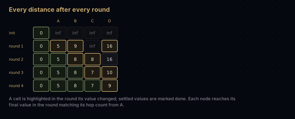
Read that table against the invariant and it lines up exactly. B is one edge from the source and settles in round 1. C's best route is A -> B -> C, two edges, settling in round 2. D needs three edges, E needs four. Round k finishes every node whose shortest path uses k edges: no more, no less.
With five nodes the longest simple path has four edges, and this graph uses all four, which is why it needs the full V − 1 = 4 rounds. Store the same six edges in path order and one round would finish the job. V − 1 is the guarantee against the worst ordering, not a prediction of the typical one.
The code
An edge list is the natural representation. Bellman-Ford never asks "what are the neighbours of this node", only "give me every edge", so a flat list of triples is all it needs.
INFINITY = float("inf")

Edge = tuple[str, str, float]

NODES = ["A", "B", "C", "D", "E"]
EDGES: list[Edge] = [
    ("D", "E", 2),
    ("C", "D", -1),
    ("B", "C", 3),
    ("A", "B", 5),
    ("A", "C", 9),
    ("B", "E", 11),
]


def bellman_ford(nodes: list[str], edges: list[Edge], source: str) -> dict[str, float]:
    """Shortest distance from source to every node, negative weights allowed.

    Relaxes every edge len(nodes) - 1 times, then runs one extra round: if any
    edge still improves after that, a negative cycle is reachable and no
    shortest path exists, so this raises instead of returning a lie.
    """
    distance = {node: INFINITY for node in nodes}
    distance[source] = 0.0

    for _ in range(len(nodes) - 1):
        changed = False
        for tail, head, weight in edges:
            if distance[tail] + weight < distance[head]:
                distance[head] = distance[tail] + weight
                changed = True
        # A round that improves nothing cannot be followed by one that does:
        # the next round would read exactly the same distances.
        if not changed:
            break

    for tail, head, weight in edges:
        if distance[tail] + weight < distance[head]:
            raise ValueError(f"negative cycle reachable via {tail}->{head}")

    return distance


distances = bellman_ford(NODES, EDGES, "A")
print(" ".join(f"{node}={distances[node]:g}" for node in NODES))A=0 B=5 C=8 D=7 E=9Fourteen lines of logic for the whole algorithm, detection included.
Reconstructing the actual route
Distances alone rarely answer the real question. One extra dictionary records, for each node, which node you arrived from when its distance last improved. Follow those pointers backwards from any target and you have the route.
def bellman_ford_paths(
    nodes: list[str], edges: list[Edge], source: str
) -> tuple[dict[str, float], dict[str, str]]:
    """Bellman-Ford that also records the edge each node was reached by."""
    distance = {node: INFINITY for node in nodes}
    distance[source] = 0.0
    parent: dict[str, str] = {}

    for _ in range(len(nodes) - 1):
        changed = False
        for tail, head, weight in edges:
            if distance[tail] + weight < distance[head]:
                distance[head] = distance[tail] + weight
                parent[head] = tail
                changed = True
        if not changed:
            break

    # Without this, a negative cycle would leave parent pointers in a loop and
    # path_to would spin forever.
    for tail, head, weight in edges:
        if distance[tail] + weight < distance[head]:
            raise ValueError(f"negative cycle reachable via {tail}->{head}")

    return distance, parent


def path_to(parent: dict[str, str], source: str, target: str) -> list[str]:
    """Walk parent pointers backwards from target, then flip the list."""
    route = [target]
    while route[-1] != source:
        if route[-1] not in parent:
            return []  # target is unreachable from source
        route.append(parent[route[-1]])
    route.reverse()
    return route


distance, parent = bellman_ford_paths(NODES, EDGES, "A")
for target in ["C", "E"]:
    route = " -> ".join(path_to(parent, "A", target))
print(f"{route} cost {distance[target]:g}")A -> B -> C cost 8
A -> B -> C -> D -> E cost 9Because every distance is final, so is every parent pointer, and together they form a tree rooted at the source: the shortest-path tree.
Detecting a negative cycle
Add one edge, E -> C with weight −8, and the loop C -> D -> E -> C sums to −1 + 2 − 8 = −7. Every lap makes every distance downstream seven units smaller, so no shortest path exists.
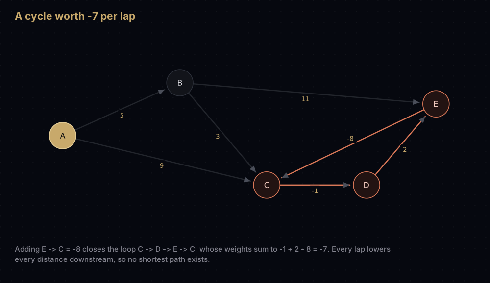
The detection round catches it immediately:
CYCLE_EDGES: list[Edge] = EDGES + [("E", "C", -8)]

try:
    bellman_ford(NODES, CYCLE_EDGES, "A")
except ValueError as error:
print(f"caught: {error}")caught: negative cycle reachable via D->EKnowing a cycle exists is often not enough, for arbitrage you want the cycle itself. Two changes get you there. First, start every distance at 0, which is the same as bolting a virtual source onto the graph with a zero-weight edge into every node; that way cycles the real source cannot reach are found too. Second, remember the last node improved in the final round and walk its parent pointers backwards V times. That is more steps than the tail leading into the cycle can be long, so you are guaranteed to land on the cycle itself.
from typing import Optional


def find_negative_cycle(nodes: list[str], edges: list[Edge]) -> Optional[list[str]]:
    """Return one negative cycle as a node list, or None if there is none.

    Every distance starts at 0, which is the same as bolting on a virtual
    source with a zero-weight edge into every node. That makes cycles the real
    source cannot reach detectable too.
    """
    distance = {node: 0.0 for node in nodes}
    parent: dict[str, str] = {}
    victim = None

    for _ in range(len(nodes)):
        victim = None
        for tail, head, weight in edges:
            # The tolerance stops floating-point noise being read as a gain.
            if distance[tail] + weight < distance[head] - 1e-12:
                distance[head] = distance[tail] + weight
                parent[head] = tail
                victim = head
        if victim is None:
            return None

    # victim may only be downstream of the cycle, so step back len(nodes)
    # times: that is more steps than the path into the cycle can be long.
    node = victim
    for _ in range(len(nodes)):
        node = parent[node]

    cycle = [node]
    walker = parent[node]
    while walker != node:
        cycle.append(walker)
        walker = parent[walker]
    cycle.append(node)
    cycle.reverse()
    return cycle


cycle = find_negative_cycle(NODES, CYCLE_EDGES)
print(" -> ".join(cycle))
weight_of = {(tail, head): weight for tail, head, weight in CYCLE_EDGES}
total = sum(weight_of[pair] for pair in zip(cycle, cycle[1:]))
print(f"cycle weight {total:g}")
print(find_negative_cycle(NODES, EDGES))D -> E -> C -> D
cycle weight -7
NoneThe same function returns None on the original graph. It names the loop starting from D rather than C, which is fine: a cycle has no canonical starting point and every rotation names the same loop.
How the code maps to the idea
INFINITY is float("inf"), not a large integer. With a sentinel like 10 ** 9, the expression 10 ** 9 + (-1) < 10 ** 9 is true, so an unreachable node "improves" to 999999999 and that nonsense spreads to its neighbours. Real infinity absorbs addition: inf + (-1) is still inf and inf < inf is false, so unreachable nodes stay untouched.
The outer loop is range(len(nodes) - 1) because that is the V − 1 from the proof: the maximum number of edges on a simple path.
The inner loop iterates the raw edge list. Any order is correct. Order only changes how many rounds you actually need, which is what the early exit exploits.
The changed flag is the early exit. If a complete pass writes nothing, the next pass would read identical distances and make identical decisions, so it would write nothing either. The fixpoint is reached. The flag must be reset at the top of each round and tested after the whole pass: testing mid-pass would abort on the first edge that happens not to improve.
The final loop is the detection round, deliberately outside the early exit. If the loop broke early the fixpoint is already reached, so the check passes instantly.
Edge cases fall out for free. A one-node graph makes range(0) empty, so no rounds run and the answer is 0. A source with no outgoing edges leaves round 1 with nothing to change, so the early exit fires after one pass. Unreachable nodes keep inf, which is the honest answer.
Here is the round-by-round table from the walkthrough, generated rather than hand-traced, with the early exit removed so every round is shown:
def rounds_of(nodes: list[str], edges: list[Edge], source: str) -> list[dict[str, float]]:
    """The full distance table after every round, for inspection."""
    distance = {node: INFINITY for node in nodes}
    distance[source] = 0.0
    history = [dict(distance)]

    for _ in range(len(nodes) - 1):
        for tail, head, weight in edges:
            if distance[tail] + weight < distance[head]:
                distance[head] = distance[tail] + weight
        history.append(dict(distance))

    return history


history = rounds_of(NODES, EDGES, "A")
print("        " + "".join(f"{node:>5}" for node in NODES))
for number, table in enumerate(history):
    label = "init" if number == 0 else f"round {number}"
print(f"{label:<8}" + "".join(f"{table[node]:>5g}" for node in NODES)) A B C D E
init 0 inf inf inf inf
round 1 0 5 9 inf 16
round 2 0 5 8 8 16
round 3 0 5 8 7 10
round 4 0 5 8 7 9Every number matches the hand trace, including the two values that were briefly wrong: D at 8 after round 2, E at 10 after round 3.
Complexity
One round costs Θ(E). It visits each of the E edges once and does constant work per edge: two dictionary lookups, an addition, a comparison, sometimes a write.
The whole algorithm is O(V · E). V − 1 rounds plus the detection round is at most V passes over the edge list, and V passes of E edges each is V · E relaxation tests. On the example graph: 4 rounds of 6 edges plus a detection round of 6, so 30 tests for five nodes.
With the early exit the cost is O((r + 1) · E), where r is the largest number of edges on any shortest path, after round r nothing can improve, so the round after it is the one that finds nothing and stops the loop. That is a ceiling, not a prediction: a favourable edge order finishes in two rounds however large r is, as the same six edges in path order do. If every node sits within three hops of the source you pay for at most four rounds however many nodes there are. Only an adversarial edge order on a long chain, like the example above, costs the full V − 1.
Space is O(V): one distance entry per node, plus one parent entry if you want routes. The edge list is O(E), but that is input, not scratch space. Nothing here needs a heap.
Against Dijkstra the gap is enormous. Dijkstra with a binary heap is O((V + E) log V). On sparse graphs where E is about 5V:
| Nodes (V) | Edges (E) | Bellman-Ford: V · E | Dijkstra: (V + E) log₂V | Ratio |
|---|---|---|---|---|
| 1,000 | 5,000 | 5,000,000 | ~60,000 | 84× |
| 10,000 | 50,000 | 500,000,000 | ~800,000 | 630× |
| 100,000 | 500,000 | 50,000,000,000 | ~10,000,000 | 5,000× |
The gap widens because Bellman-Ford is quadratic in V at fixed edge density while Dijkstra is barely worse than linear. On a dense graph where E approaches V², Bellman-Ford is O(V³): the same bound Floyd-Warshall achieves for all pairs. Negative weights cost you roughly three orders of magnitude at real scale; pay it only when you must. The Big O post has the full counting argument behind these bounds.
The queue optimisation, and its reputation
Most of the work in a round is wasted: an edge can only improve anything if the distance at its tail changed since that edge was last examined. SPFA, the Shortest Path Faster Algorithm, exploits exactly that. Keep a queue of nodes whose distance changed, pop one, relax only its outgoing edges, and push any neighbour that improved and is not already queued. It wants an adjacency list rather than an edge list, and collections.deque is the right container.
On ordinary graphs it is dramatically faster, often close to a single pass over the edges. But the worst case is still O(V · E) and it is not hard to hit: grid-shaped graphs with the right weights reliably push it to the bound, which is why competitive programmers treat SPFA as unsafe under a strict time limit. It also loses the clean "after round k" invariant, so cycle detection changes: count relaxations per node and declare a cycle when any node hits V. Reach for it when profiling says the plain version is too slow, not by default.
When to use it, and when not to
Use it when weights can be negative and you need single-source shortest paths. Nothing simpler covers that case.
Use it when the question is "is there a negative cycle at all": feasibility checks, arbitrage scans. Start every distance at 0 and the answer covers the whole graph, not just what one source reaches.
Use it when nobody has the whole graph. Relaxation is purely local: a node needs only its own distance, its neighbours' advertised distances and its own link weights. That is why the algorithm survives in distributed routing.
Use it when you need a hop limit. Round k solves exactly the "at most k edges" problem, so running only k rounds answers "cheapest route using at most k edges": the airline problem of the cheapest flight with at most two stops. One catch: relax against a snapshot of the previous round's distances, or improvements chain within a round and quietly exceed the limit.
Do not use it when every weight is non-negative. Use Dijkstra and take the three orders of magnitude. Here is what ignoring that looks like on the trap graph from earlier:
import heapq

TRAP_NODES = ["S", "A", "B", "T"]
TRAP_EDGES: list[Edge] = [
    ("S", "A", 1),
    ("S", "B", 3),
    ("B", "A", -5),
    ("A", "T", 1),
]


def dijkstra(nodes: list[str], edges: list[Edge], source: str) -> dict[str, float]:
    """Textbook Dijkstra: settle the closest unsettled node, then relax it."""
    outgoing: dict[str, list[tuple[str, float]]] = {node: [] for node in nodes}
    for tail, head, weight in edges:
        outgoing[tail].append((head, weight))

    distance = {node: INFINITY for node in nodes}
    distance[source] = 0.0
    settled: set[str] = set()
    queue = [(0.0, source)]

    while queue:
        current, node = heapq.heappop(queue)
        if node in settled:
            continue
        settled.add(node)  # Dijkstra's bet: this distance is final
        for head, weight in outgoing[node]:
            if current + weight < distance[head]:
                distance[head] = current + weight
                heapq.heappush(queue, (distance[head], head))

    return distance


greedy = dijkstra(TRAP_NODES, TRAP_EDGES, "S")
correct = bellman_ford(TRAP_NODES, TRAP_EDGES, "S")
print("dijkstra     " + " ".join(f"{n}={greedy[n]:g}" for n in TRAP_NODES))
print("bellman-ford " + " ".join(f"{n}={correct[n]:g}" for n in TRAP_NODES))dijkstra S=0 A=-2 B=3 T=2
bellman-ford S=0 A=-2 B=3 T=-1Note the shape of the failure. Dijkstra's answer for A is right: the relaxation still wrote −2 into the table. It is T that is wrong, because by the time A improved it had already been settled and expanded, so nothing downstream ever heard about it. Wrong answers from Dijkstra on negative edges are quiet and partial, which is the worst kind.
Do not use it on a directed acyclic graph. Process nodes in topological order and one pass suffices, O(V + E), negative weights and all. A DAG always has such an order, and relaxing edges in it settles every node in a single sweep. It is the ordering that buys this, not the absence of cycles: plain Bellman-Ford on a DAG whose edges are stored back to front still needs all V − 1 rounds.
Do not use it for all pairs. Floyd-Warshall does every pair in O(V³) with simpler code. On sparse graphs Johnson's algorithm is better still: one Bellman-Ford run from a virtual source produces a potential per node, which reweights every edge to be non-negative while preserving which paths are shortest, and then Dijkstra runs from every node.
Do not use it on an undirected graph with a negative edge. An undirected negative edge is a negative cycle: walk back and forth across it forever and the total falls without limit. The question has no answer, and any implementation that returns one is wrong.
Do not use it on an unweighted graph. Breadth-first search gives shortest paths in O(V + E).
Where it shows up in the real world
RIP, the Routing Information Protocol. RIP (RFC 2453 for version 2) is distance-vector routing, and distance-vector routing is Bellman-Ford run by a network of machines, none of which can see the whole graph. Each router keeps a vector of costs to every destination, broadcasts it to its directly connected neighbours every 30 seconds, and on receiving a neighbour's vector recomputes its own cost to each destination as the minimum over neighbours of (cost to that neighbour + the cost that neighbour advertises). That recomputation is the relaxation step, distributed.
The bound on rounds shows up in the protocol as a hard number: RIP's maximum metric is 15 hops and 16 means "unreachable". Infinity is a literal small integer. That looks crippling until you see the reason: it bounds the count-to-infinity problem, where two routers keep incrementing each other's stale estimate after a link dies, each believing the other still has a route. Capping infinity at 16 makes that terminate in bounded time instead of never.
Modern networks mostly run link-state protocols instead: OSPF and IS-IS give every router the full topology and let it run Dijkstra locally. Between autonomous systems, BGP is a path-vector protocol: a descendant of distance-vector that carries the entire AS path in each advertisement, so loops are detected outright rather than counted to.
Currency arbitrage. This is the best use of negative-cycle detection, because the transformation is genuinely elegant.
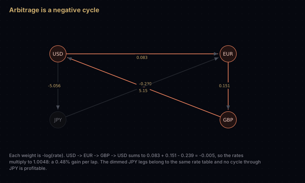
Exchange rates multiply along a chain. Trade USD to EUR at 0.92, EUR to GBP at 0.86, GBP back to USD at 1.27, and one dollar becomes 0.92 × 0.86 × 1.27 = 1.004824 dollars. Any cycle whose rates multiply to more than 1 is free money.
Shortest-path algorithms add along a path. So you need a function that turns multiplication into addition, and that function is the logarithm: log(r₁ × r₂ × r₃) = log r₁ + log r₂ + log r₃.
Now chase the inequality. Profit means the product exceeds 1. Take logs of both sides: the sum of the logs exceeds 0. Negate: the sum of the negated logs falls below 0. So define the weight of the edge from currency u to currency v as −log(rate), and a profitable trading cycle becomes precisely a cycle of negative total weight: exactly what the extra round already hunts for. The negation is not cosmetic: relaxation only ever chases minima, so a positive cycle would be invisible to it.
from math import log

RATES = {
    ("USD", "EUR"): 0.92,
    ("EUR", "USD"): 1.08,
    ("USD", "GBP"): 0.786,
    ("GBP", "USD"): 1.27,
    ("USD", "JPY"): 157.0,
    ("JPY", "USD"): 0.0063,
    ("EUR", "GBP"): 0.86,
    ("GBP", "EUR"): 1.16,
    ("EUR", "JPY"): 170.0,
    ("JPY", "EUR"): 0.0058,
}

CURRENCIES = ["USD", "EUR", "GBP", "JPY"]
RATE_EDGES: list[Edge] = [(a, b, -log(rate)) for (a, b), rate in RATES.items()]

loop = find_negative_cycle(CURRENCIES, RATE_EDGES)
print(" -> ".join(loop))
product = 1.0
for pair in zip(loop, loop[1:]):
    product *= RATES[pair]
print(f"1 unit becomes {product:.6f} — a {(product - 1) * 100:.3f}% gain")EUR -> GBP -> USD -> EUR
1 unit becomes 1.004824 — a 0.482% gainTen rates, one profitable loop, found by the same function that found D -> E -> C -> D. Starting every distance at 0 is what makes it work: the profitable cycle need not involve whichever currency you happen to hold.
Be honest about the limits. Quoted rates are mid-market; you trade at the bid or the ask, and every leg of the loop pays that spread. Add fees and the fact that the quotes were not executable at the same instant, and the opportunity is normally gone before you can act. The 0.48% above is a teaching number, chosen so the arithmetic is visible: a gap that wide in a liquid major pair would not survive the second it appeared. The technique is real and lives in exchange monitoring and risk tooling; the free money mostly is not.
Systems of difference constraints. Inequalities of the form x_j - x_i <= c map straight onto a graph: one node per variable, one edge from i to j of weight c. Bellman-Ford from a virtual source either returns distances that satisfy every constraint or reports a negative cycle, which is a proof that the constraints contradict each other. Schedulers and timing analysers use this, and it is a good reminder that shortest-path problems are often not about paths at all.
What to reach for in Python. There is no Bellman-Ford in the standard library: heapq gives you enough to hand-write Dijkstra and the batteries stop there. For real work use SciPy's scipy.sparse.csgraph.bellman_ford and johnson, or NetworkX's bellman_ford_predecessor_and_distance and find_negative_cycle.
Common mistakes
Using a large integer as infinity. 10 ** 9 + (-5) < 10 ** 9 is true, so an unreachable node improves to a garbage value and advertises it onwards. Use float("inf"), or explicitly skip edges whose tail is still unreached. In C++ the same bug also overflows INT_MAX into negative numbers.
Skipping the detection round. Without it, a graph with a negative cycle returns numbers that look plausible and mean nothing. The V − 1 rounds do not fail loudly; they just stop on a problem with no answer.
Assuming detection tells you which nodes are affected. It tells you a cycle exists. To find every node whose true distance is −infinity, mark the heads of all still-relaxable edges and flood that mark forward with a BFS or DFS.
Detecting cycles from a single source. A negative cycle in a component the source cannot reach is never found. If the question is "does this graph contain one anywhere", initialise every distance to 0.
Testing the changed flag inside the edge loop. It must be reset at the start of each round and tested only after a full pass; breaking on the first non-improving edge stops the algorithm almost immediately on almost every graph.
Reconstructing a path before checking for cycles. With a negative cycle present, parent pointers can form a loop and the backwards walk never terminates. Run the detection round first, or bound the walk to V steps.
Practice
- Print the round number in which each node reaches its final distance, and check it equals the number of edges on that node's shortest path.
- Replace the
raisewith a return value: the set of nodes whose true distance is −infinity, found by marking the heads of still-relaxable edges and flooding forward. - Build a chain of eight nodes, store its edges in reverse order and count the rounds the early-exit version runs; re-run with the edges in path order and count again.
- Add a hop limit: return the cheapest route to a target using at most k edges, by running k rounds against a snapshot of the previous round's distances.
- Implement SPFA with
collections.dequeand a per-node relaxation counter that reports a negative cycle when any node is relaxed V times, then confirm it agrees with the code here on both example graphs.
Summary
Bellman-Ford trades speed for the one thing Dijkstra cannot do. It relaxes every edge V − 1 times because a shortest path is simple and a simple path has at most V − 1 edges, and after round k every node whose best route uses k edges is already correct. One extra round then tests, exactly and without false positives, whether a negative cycle makes the question unanswerable, which is what turns it into an arbitrage detector once the edges carry negated logs.
| Difficulty | Hard |
| Best case | O(E) — one round changes nothing and the early exit fires |
| Average case | O((r + 1) · E) — r is the most edges on any shortest path |
| Worst case | O(V · E) — V − 1 rounds plus detection, each scanning every edge |
| Space | O(V) — one distance and one parent entry per node, no heap |
| Handles negative weights | Yes — the entire reason it exists |
| Detects negative cycles | Yes — one extra round, exact in both directions |
| Data structure | Edge list; no adjacency list or priority queue needed |
| Use it when | Weights can go below zero, or a negative cycle must be found |
| Avoid it when | All weights are non-negative — Dijkstra is O((V + E) log V) |
| Real-world use | RIP distance-vector routing, currency arbitrage scans, Johnson's algorithm |
| Python equivalent | None in the standard library; scipy.sparse.csgraph.bellman_ford, nx.find_negative_cycle |
The algorithm is fourteen lines. The proof of the loop bound is the real content, and it is worth being able to reproduce from memory: it is the cleanest case in this series of a complexity bound that falls out of a structural fact about the problem rather than out of counting a loop.
Keep reading
- Dijkstra's Algorithm — the faster answer whenever every weight is non-negative, and the one to reach for first.
- Floyd-Warshall — every pair of nodes at once, negative weights included, in three nested loops.
- Topological Sort — the linear-time shortest path on a DAG, which beats Bellman-Ford outright.
- Graphs in Python — edge lists, adjacency lists and matrices, and why this algorithm wants the first.
- Breadth-First Search — shortest paths when every edge costs the same, in O(V + E).


