You have a set of sites and a price list of possible links between them. Every site must end up connected to every other site, directly or through the others, and you want to pay as little as possible in total. That is the minimum spanning tree problem, and it is one of the rare places where the greedy instinct — always grab the cheapest thing available — is not a decent heuristic but a provably optimal algorithm.
Two algorithms solve it, both from the mid-1950s, and both are still what you would write today. Kruskal's sorts every edge by weight and walks the sorted list, taking each edge unless it closes a cycle. Prim's grows one connected blob outwards from a starting node, always swallowing the cheapest edge that leaves the blob. They look nothing alike, they add edges in completely different orders, and they always arrive at the same total cost.
The reason both work is a single fact called the cut property. Most treatments state it and move on. This one proves it with an exchange argument short enough to hold in your head, because once you have that argument the two algorithms stop being separate tricks and become one idea applied in two orders. After that: full implementations, both traced on the same graph, the counting arguments behind O(E log E) and O(E log V), and a straight answer on which to reach for.
The idea
What a spanning tree is
Start with an undirected graph: vertices joined by edges, each edge carrying a weight, and no direction on any edge — if A links to B then B links to A at the same price. A spanning tree is a subset of the edges that keeps every vertex connected to every other and contains no cycles. A minimum spanning tree is the spanning tree whose weights add up to the smallest possible total.
Every spanning tree has exactly V − 1 edges, and that is not a definition, it is a counting argument. Begin with V vertices and no edges at all: you have V separate components. Now add edges one at a time. An edge whose two endpoints sit in different components fuses them, dropping the component count by one. An edge whose endpoints sit in the same component adds nothing: both ends were already reachable from each other, so the edge closes a cycle and the count stays put. To get from V components down to 1 you therefore need exactly V − 1 of the first kind. One fewer and something is unreachable; one more and you have a cycle. Both algorithms below use that number as their stopping rule.
Here is the graph this post works through. Seven vertices, ten edges, every weight distinct:
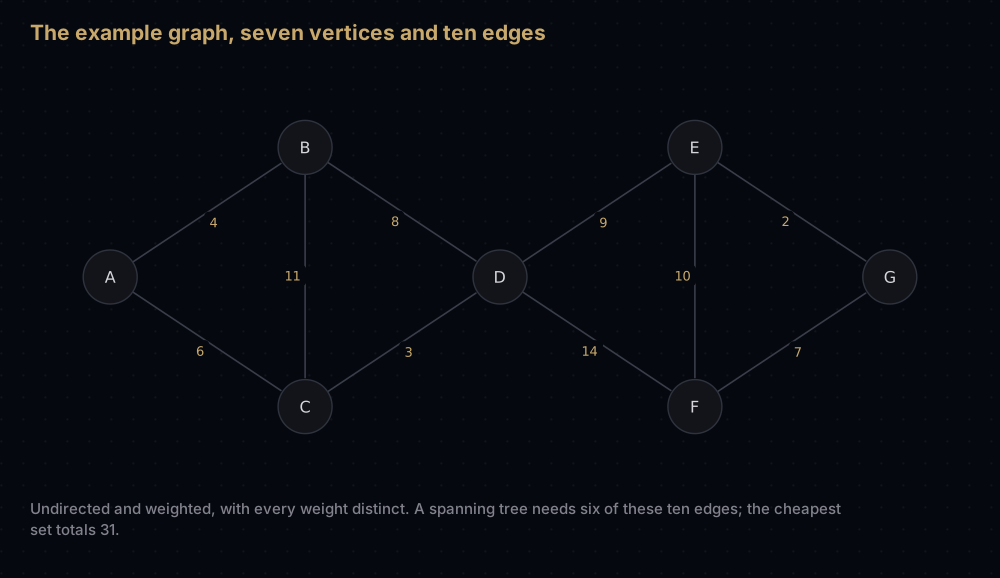
A spanning tree here needs six of those ten edges, and there are exactly 64 different six-edge sets that connect everything. You want the cheapest one.
The cut property, and why greedy is safe here
A cut is any way of splitting the vertices into two non-empty groups. An edge crosses the cut when one endpoint lands in each group.
Cut property. For any cut of the graph, the cheapest edge crossing that cut belongs to some minimum spanning tree. If it is strictly cheaper than every other crossing edge, it belongs to every minimum spanning tree.
Here is why. Read it slowly: it is the entire justification for both algorithms.
Let e be a cheapest edge crossing some cut, with endpoint u on one side and v on the other. Suppose some minimum spanning tree T leaves e out. T connects everything, so it contains a path from u to v. That path starts on one side of the cut and ends on the other, so somewhere along it there is an edge f that crosses the cut too.
Now do the exchange: delete f from T and add e. Deleting f splits T into exactly two pieces, one holding u and one holding v: that follows because f lies on the only u-to-v path in a tree, so cutting it separates them. Adding e reconnects those two pieces, because e has one endpoint in each. The result still has V − 1 edges and still reaches every vertex, so it is a spanning tree, and its weight is the weight of T, minus f, plus e.
Since e is a cheapest crossing edge and f also crosses, the weight of e is at most the weight of f. So the new tree weighs no more than T. T was minimum, so the new tree is minimum too, and it contains e. And if e is strictly cheaper than f, the new tree is strictly lighter, which contradicts T being minimum in the first place. No minimum spanning tree could have left e out.
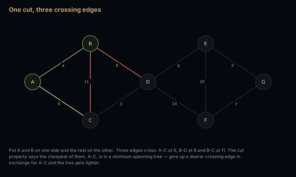
That is all either algorithm does. Find a cut, take its cheapest crossing edge, repeat V − 1 times.
- Prim's cut is obvious: the tree built so far on one side, everything else on the other. The cheapest edge leaving the tree is by definition the cheapest crossing edge.
- Kruskal's cut is subtler. When it accepts an edge joining
uandv, take the cut to be "the component currently containingu" against everything else. Any other edge crossing that cut has not been examined yet: if it had been, it would have joined two different components and so been accepted, which would have made the component bigger than it is. Unexamined means later in sorted order, which means at least as expensive. So the edge Kruskal is holding is a cheapest crossing edge of that cut.
Watching it work
Kruskal: sort, then filter
Sorted by weight, the ten edges are: E-G (2), C-D (3), A-B (4), A-C (6), F-G (7), B-D (8), D-E (9), E-F (10), B-C (11), D-F (14).
Walk them in that order, keeping a forest of accepted edges:
- E-G at 2. E and G are each alone. Accept. Six components remain.
- C-D at 3. Also both alone. Accept. Five components.
- A-B at 4. Accept. Four components: A-B, C-D, E-G, and F on its own.
- A-C at 6. A sits in the A-B fragment, C in the C-D fragment. Different, so accept, and the two fragments fuse into A-B-C-D. Three components.
- F-G at 7. F is alone, G is with E. Accept. Two components: A-B-C-D and E-F-G.
- B-D at 8. Both B and D are already inside A-B-C-D. Reject — this edge would close the cycle B to A to C to D and back to B.
- D-E at 9. D is in one component, E in the other. Accept, and everything is now connected. That is the sixth edge, which is V − 1, so nothing after it could possibly be accepted. Stop.
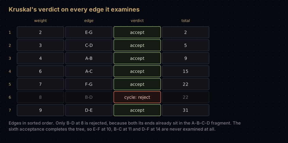
Total: 2 + 3 + 4 + 6 + 7 + 9 = 31. Notice what the intermediate states looked like, for most of the run the accepted edges formed several disconnected fragments, not a tree. Kruskal maintains a forest and only merges it into one piece on the last accepted edge. The three most expensive edges were never even examined.
Prim: grow one blob
Same graph, start at A. The tree begins as the single vertex A, and each step takes the cheapest edge with exactly one endpoint inside it.
- Crossing edges: A-B (4), A-C (6). Take A-B. Tree is A, B. Total 4.
- Crossing: A-C (6), B-D (8), B-C (11). Take A-C. Tree is A, B, C. Total 10.
- Crossing: C-D (3), B-D (8). Take C-D. Tree is A, B, C, D. Total 13.
- Crossing: D-E (9), D-F (14). Take D-E. Total 22.
- Crossing: E-G (2), E-F (10), D-F (14). Take E-G. Total 24.
- Crossing: G-F (7), E-F (10), D-F (14). Take G-F. Total 31, six edges, done.
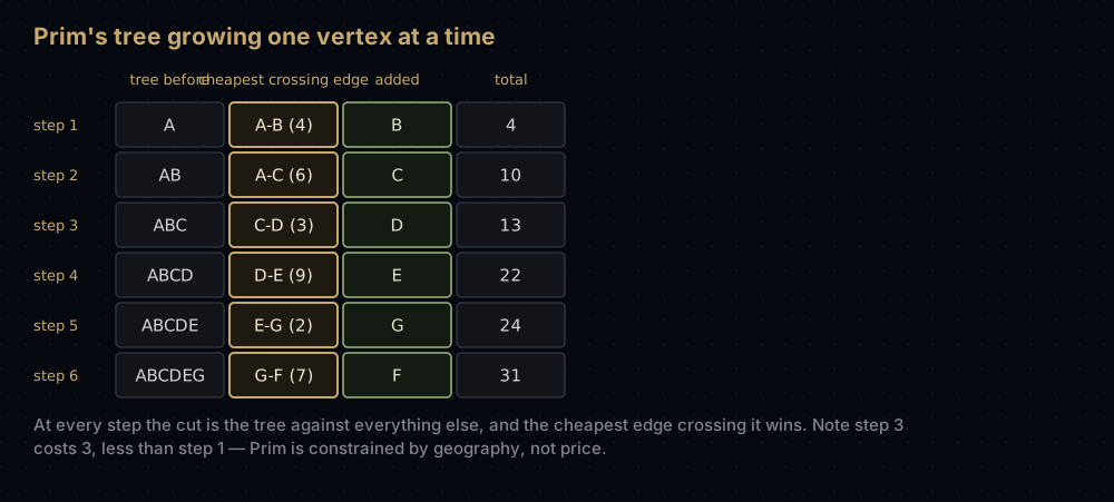
Thirty-one again, and in fact the same six edges. The order is completely different: Kruskal accepted them at costs 2, 3, 4, 6, 7, 9 (sorted, necessarily) while Prim took them at 4, 6, 3, 9, 2, 7. Prim's third pick costs less than its first, which Kruskal can never do. Prim is constrained by geography, Kruskal by price.
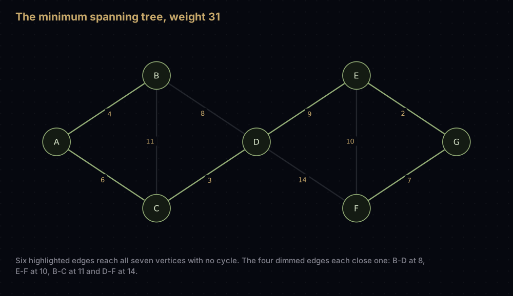
The four losing edges are B-D (8), E-F (10), B-C (11) and D-F (14). Each one, added to the tree, would close a cycle. Because every weight in this graph is distinct, this tree is the only minimum one: ties are the only way to get more than one answer, and there is a demonstration of that below.
The code
Represent the graph as a flat list of (weight, u, v) tuples. Putting the weight first is the single most load-bearing detail in this post: it means sorted(edges) sorts by cost, and it means a heap of edges pops the cheapest one, with no key function anywhere.
Kruskal, the obvious way first
The algorithm needs one thing it does not get for free: a test for "would this edge close a cycle?". The obvious implementation searches the edges accepted so far.
from __future__ import annotations

import heapq

# An undirected weighted graph as a flat list of (weight, u, v) edges. Weight
# comes first on purpose: sorting a list of these sorts by cost, which is the
# only ordering either algorithm ever needs.
Edge = tuple[int, str, str]

NODES = ["A", "B", "C", "D", "E", "F", "G"]
EDGES: list[Edge] = [
    (4, "A", "B"),
    (6, "A", "C"),
    (11, "B", "C"),
    (8, "B", "D"),
    (3, "C", "D"),
    (9, "D", "E"),
    (14, "D", "F"),
    (10, "E", "F"),
    (2, "E", "G"),
    (7, "F", "G"),
]


def show(tree: list[Edge]) -> str:
    """Format a tree as 'A-B(4)' pieces, in the order the algorithm chose them."""
    return "  ".join(f"{u}-{v}({weight})" for weight, u, v in tree)


def reaches(chosen: list[Edge], start: str, goal: str) -> bool:
    """Is goal already reachable from start using only the edges chosen so far?"""
    seen = {start}
    stack = [start]
    while stack:
        node = stack.pop()
        if node == goal:
            return True
        for _, a, b in chosen:
            if a == node and b not in seen:
                seen.add(b)
                stack.append(b)
            elif b == node and a not in seen:
                seen.add(a)
                stack.append(a)
    return False


def naive_kruskal(nodes: list[str], edges: list[Edge]) -> tuple[list[Edge], int]:
    """Kruskal with the obvious cycle test: search the forest built so far."""
    tree: list[Edge] = []
    total = 0
    for weight, u, v in sorted(edges):
        if not reaches(tree, u, v):
            tree.append((weight, u, v))
            total += weight
    return tree, total


naive_tree, naive_total = naive_kruskal(NODES, EDGES)
print("edges:", show(naive_tree))
print("total:", naive_total)edges: E-G(2) C-D(3) A-B(4) A-C(6) F-G(7) D-E(9)
total: 31Correct, and too slow. Each reaches call runs a graph search, and a forest on V vertices holds fewer than V edges, so even a well-implemented search costs O(V) per call. Run it on all E edges and Kruskal lands at O(E · V): worse than the sort it is built on. The version above is worse still, because it rescans the whole chosen list for every vertex it visits.
The cycle test, done properly
A disjoint-set forest, also called union-find, answers "are these two things already connected?" in effectively constant time. Every label points at a parent; follow parents until you reach one that points at itself, and that root identifies the component. Merging two components is one pointer write, from one root to the other.
Two refinements make it fast. Union by size always hangs the smaller tree under the larger root, so no chain gets long. Path compression re-points every node it walked past straight at the root, so the next lookup is one hop. Together they give an amortised cost per operation of O(α(V)), where α is the inverse Ackermann function: a function that grows so slowly it is at most 4 for any input that fits in a computer. Treat it as constant. Union-find has its own post if you want that bound derived properly.
class DisjointSet:
    """Union-find over labels, with union by size and path compression.

    parent[x] is x's parent, and x is a root when it is its own parent.
    size[r] counts the labels in the tree rooted at r, and is only meaningful
    while r really is a root.
    """

    def __init__(self, items: list[str]) -> None:
        self.parent = {item: item for item in items}
        self.size = {item: 1 for item in items}

    def find(self, item: str) -> str:
        """Return the root of item's component, flattening the path behind us."""
        root = item
        while self.parent[root] != root:
            root = self.parent[root]

        # Second walk over the same path: everything on it now points straight
        # at the root, so the next find on any of them costs one hop.
        while self.parent[item] != root:
            next_item = self.parent[item]
            self.parent[item] = root
            item = next_item
        return root

    def union(self, a: str, b: str) -> bool:
        """Merge two components. False means they were already the same one."""
        root_a, root_b = self.find(a), self.find(b)
        if root_a == root_b:
            return False

        # Hang the smaller tree under the bigger root, so the labels that gain
        # a level are the ones in the smaller half.
        if self.size[root_a] < self.size[root_b]:
            root_a, root_b = root_b, root_a
        self.parent[root_b] = root_a
        self.size[root_a] += self.size[root_b]
        return True


def kruskal(nodes: list[str], edges: list[Edge]) -> tuple[list[Edge], int]:
    """Minimum spanning tree: take edges cheapest first, skipping the cycles."""
    forest = DisjointSet(nodes)
    tree: list[Edge] = []
    total = 0

    for weight, u, v in sorted(edges):
        # union() returns False exactly when u and v already share a root,
        # which is exactly when this edge would close a cycle.
        if forest.union(u, v):
            tree.append((weight, u, v))
            total += weight
            if len(tree) == len(nodes) - 1:
                break  # V - 1 edges already span everything

    return tree, total


def kruskal_traced(nodes: list[str], edges: list[Edge]) -> None:
    """Kruskal again, printing the verdict on every edge it looks at."""
    forest = DisjointSet(nodes)
    accepted = 0
    total = 0

    for weight, u, v in sorted(edges):
        if forest.union(u, v):
            accepted += 1
            total += weight
            print(f"{weight:>3}  {u}-{v}  accept   running total {total}")
        else:
            print(f"{weight:>3}  {u}-{v}  reject   {u} and {v} are already joined")
        if accepted == len(nodes) - 1:
            print(f"     stop     {accepted} edges span {len(nodes)} nodes")
            break


kruskal_traced(NODES, EDGES) 2 E-G accept running total 2
3 C-D accept running total 5
4 A-B accept running total 9
6 A-C accept running total 15
7 F-G accept running total 22
8 B-D reject B and D are already joined
9 D-E accept running total 31
stop 6 edges span 7 nodesThat is the walkthrough from above, line for line, including the single rejection at weight 8.
Prim on a heap
Prim needs a different question answered: "what is the cheapest edge leaving the tree right now?". That is a priority queue, and Python's heapq is one: a list kept in min-heap order, with heappush and heappop both costing O(log n).
The bookkeeping trick is the same one Dijkstra's algorithm uses. Rather than trying to remove edges from the heap when they stop being useful, leave them there and discard them on the way out. An edge is useless once both its endpoints are inside the tree, and one set membership test catches that.
def build_adjacency(nodes: list[str],
                    edges: list[Edge]) -> dict[str, list[tuple[int, str]]]:
    """Each node mapped to its (weight, neighbour) pairs, in both directions."""
    adjacency: dict[str, list[tuple[int, str]]] = {node: [] for node in nodes}
    for weight, u, v in edges:
        adjacency[u].append((weight, v))
        adjacency[v].append((weight, u))
    return adjacency


def prim(nodes: list[str], edges: list[Edge], start: str) -> tuple[list[Edge], int]:
    """Minimum spanning tree grown outwards from one node, using a heap.

    The heap holds every known edge from the tree to a vertex outside it, so
    its smallest entry is the cheapest edge crossing the cut between the tree
    and the rest of the graph. The cut property says that edge is always safe.
    """
    adjacency = build_adjacency(nodes, edges)
    in_tree = {start}
    frontier = [(weight, start, neighbour) for weight, neighbour in adjacency[start]]
    heapq.heapify(frontier)
    tree: list[Edge] = []
    total = 0

    while frontier and len(tree) < len(nodes) - 1:
        weight, inside, outside = heapq.heappop(frontier)
        if outside in in_tree:
            continue  # stale: something cheaper already pulled it in

        in_tree.add(outside)
        tree.append((weight, inside, outside))
        total += weight
        for next_weight, neighbour in adjacency[outside]:
            if neighbour not in in_tree:
                heapq.heappush(frontier, (next_weight, outside, neighbour))

    return tree, total


def prim_traced(nodes: list[str], edges: list[Edge], start: str) -> None:
    """Prim again, printing every heap pop including the stale ones."""
    adjacency = build_adjacency(nodes, edges)
    in_tree = {start}
    frontier = [(weight, start, neighbour) for weight, neighbour in adjacency[start]]
    heapq.heapify(frontier)
    chosen = 0
    total = 0

    while frontier and chosen < len(nodes) - 1:
        weight, inside, outside = heapq.heappop(frontier)
        if outside in in_tree:
            print(f"{weight:>3}  {inside}-{outside}  skip     "
                  f"{outside} is in the tree already")
            continue

        in_tree.add(outside)
        chosen += 1
        total += weight
        print(f"{weight:>3}  {inside}-{outside}  take     tree = "
              f"{''.join(sorted(in_tree))}, total {total}")
        for next_weight, neighbour in adjacency[outside]:
            if neighbour not in in_tree:
                heapq.heappush(frontier, (next_weight, outside, neighbour))


prim_traced(NODES, EDGES, "A") 4 A-B take tree = AB, total 4
6 A-C take tree = ABC, total 10
3 C-D take tree = ABCD, total 13
8 B-D skip D is in the tree already
9 D-E take tree = ABCDE, total 22
2 E-G take tree = ABCDEG, total 24
7 G-F take tree = ABCDEFG, total 31Seven pops for six edges. The one skip is B-D at weight 8, pushed when B joined and D was still outside, popped after C-D at weight 3 had already brought D in.
One graph, two algorithms
kruskal_tree, kruskal_total = kruskal(NODES, EDGES)
prim_tree, prim_total = prim(NODES, EDGES, "A")

print("kruskal:", show(kruskal_tree))
print("prim:   ", show(prim_tree))
print("totals: ", kruskal_total, prim_total)
print("same edges:", {frozenset((u, v)) for _, u, v in kruskal_tree}
                     == {frozenset((u, v)) for _, u, v in prim_tree})

# Two inputs that have no spanning tree at all, handled without a special case.
islands: list[Edge] = [(1, "A", "B"), (5, "C", "D")]
island_tree, island_total = kruskal(["A", "B", "C", "D"], islands)
print("disconnected:", show(island_tree), "->", len(island_tree), "edges, not 3")
print("single node: ", kruskal(["A"], []), prim(["A"], [], "A"))kruskal: E-G(2) C-D(3) A-B(4) A-C(6) F-G(7) D-E(9)
prim: A-B(4) A-C(6) C-D(3) D-E(9) E-G(2) G-F(7)
totals: 31 31
same edges: True
disconnected: A-B(1) C-D(5) -> 2 edges, not 3
single node: ([], 0) ([], 0)How the code maps to the idea
union() returning a boolean is the entire cycle test. True means the edge joined two separate components and belongs in the tree; False means both endpoints already shared a root, so the edge closes a cycle. There is no graph search anywhere in kruskal.
The break at V − 1 edges is the counting argument from the first section, spent. Once six edges have been accepted on seven vertices, everything is connected, so every remaining edge would close a cycle. On this graph that skips the three most expensive edges entirely.
in_tree in prim is one side of the cut. The heap holds the crossing edges it knows about, so heappop returns the cheapest crossing edge, which the cut property licenses it to take. That is the correctness proof and the implementation lined up one to one.
Stale heap entries are the price of not having decrease_key. An entry is pushed only when its far end is outside the tree, but that vertex can be pulled in by something cheaper before the entry pops, and then the entry is garbage, which is exactly what happened to B-D. Discarding it costs one set lookup. On this graph ten entries ever enter the heap, seven get popped, one of those is stale, and three are still sitting there unexamined when the tree fills up.
Edge cases fall out without special code. A disconnected graph gives Kruskal a spanning forest (the run above returns 2 edges for 4 vertices, not 3), so if a spanning tree is required, check len(tree) == len(nodes) - 1 and treat anything less as failure. Prim on a disconnected graph is worse: it silently returns the tree of the start vertex's component only. A single vertex needs zero edges, and both functions return an empty tree with total 0. A self-loop is rejected by union and never pushed by Prim. Parallel edges between the same pair are harmless: the cheaper is accepted and the dearer closes a cycle.
When the two disagree
Both algorithms always report the same total weight, because the minimum is the minimum. When weights tie, though, they can return different trees, and so can Prim run twice from different starting vertices. Take a four-vertex square with two cheap sides and two dear ones:
SQUARE_NODES = ["A", "B", "C", "D"]
SQUARE: list[Edge] = [(1, "A", "B"), (2, "B", "C"), (1, "C", "D"), (2, "A", "D")]

square_tree, square_total = kruskal(SQUARE_NODES, SQUARE)
print(f"kruskal      {show(square_tree)}   total {square_total}")
for node in SQUARE_NODES:
    grown, grown_total = prim(SQUARE_NODES, SQUARE, node)
print(f"prim from {node} {show(grown)} total {grown_total}")kruskal A-B(1) C-D(1) A-D(2) total 4
prim from A A-B(1) A-D(2) D-C(1) total 4
prim from B B-A(1) A-D(2) D-C(1) total 4
prim from C C-D(1) C-B(2) B-A(1) total 4
prim from D D-C(1) C-B(2) B-A(1) total 4Both weight-1 edges are in every answer. Exactly one of the two weight-2 edges gets in, and which one depends on tie-breaking: Kruskal and Prim-from-A settle on A-D, Prim-from-C settles on B-C. Total 4 either way.
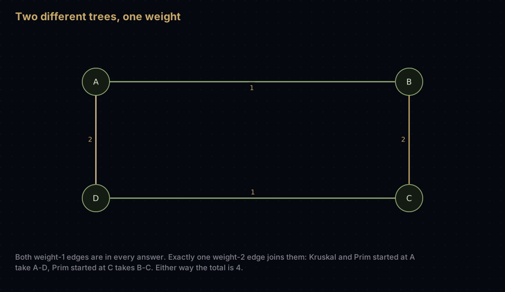
The rule is worth remembering: distinct edge weights guarantee a unique minimum spanning tree; equal weights allow several, all of the same total weight. If a test asserts on the exact edge set rather than the total, it will pass or fail on the whim of your sort's tie-break.
Complexity
Kruskal
Three costs, and one of them dominates.
Sorting E edges: O(E log E). In CPython that is list.sort, which is Timsort running in C.
One union per edge: E calls. With union by size and path compression each call is O(α(V)) amortised, and α is at most 4 for any V you can store. So the union-find phase is O(E α(V)), which is linear in E for every practical purpose.
Setting up the structure: O(V), one dictionary entry per vertex.
Add them: O(E log E + E α(V) + V), and the sort swallows the rest. Kruskal is O(E log E). Because a simple graph has at most V(V − 1) / 2 edges, log E < 2 log V, so O(E log E) can equally be written O(E log V): the two forms describe the same bound.
That log factor is entirely the sort, which means it disappears when the sort does. If the edges arrive pre-sorted, or the weights are small integers you can counting-sort or radix-sort in O(E), the whole algorithm drops to O(E α(V)) — effectively linear.
Prim
Building the adjacency lists: O(V + E), one pass over the edges writing two entries each.
Heap pushes: at most 2E. Each vertex enters the tree exactly once, and when it does, its adjacency list is scanned and at most one entry is pushed per neighbour. Summing degrees over all vertices gives 2E, so 2E is the ceiling on pushes across the entire run, no matter how the graph is shaped.
Heap pops: at most 2E, because you cannot pop more than you push.
Cost per heap operation: O(log H) where H is the heap size, and H never exceeds 2E. Since E is at most V², log(2E) is O(log V).
Multiply out: Prim on a binary heap is O(E log V). Note the heap size, not the vertex count, is what the log measures — lazy deletion trades a bigger heap for simpler code, and 2E instead of V inside a logarithm changes nothing asymptotically.
Which is actually faster
Both are O(E log V), so the choice comes down to shape and constants.
On a dense graph, drop the heap. Prim with an adjacency matrix and a plain linear scan for the nearest outside vertex runs V rounds, each scanning V candidates: O(V²), with no heap and no stale entries. When E is close to V², that beats O(E log V) = O(V² log V) outright. Same trade-off as Dijkstra, same reason.
On a sparse graph, Kruskal's one sort is cheap and its inner loop is a couple of dictionary lookups, where Prim pays heap work per edge.
Space is O(V + E) for both. Kruskal holds the edge list plus two dictionaries of size V. Prim holds the adjacency lists plus a heap of up to 2E entries.
Neither has a meaningful best case. Every edge has to be looked at at least once: an edge you never examine could have been the cheapest crossing edge of some cut, and skipping it could cost you the optimum. Kruskal can stop accepting early, as it did above, but the sort has already touched everything. If early exit matters, replace the sort with heapq.heapify — O(E) — and pop edges one at a time, so you only pay log E for the edges you actually reach.
Better bounds exist, and mostly you should not implement them. Prim on a Fibonacci heap is O(E + V log V), but the constant factors are large enough that a binary heap usually wins on graphs of realistic size. Karger, Klein and Tarjan's randomised algorithm runs in expected linear time and is intricate enough that almost nobody ships it. Borůvka's algorithm is the exception: the same O(E log V) bound, but each of its rounds is independent per component, which is why parallel and GPU minimum spanning tree implementations are built on Borůvka rather than on either algorithm here.
When to use it, and when not to
Reach for Kruskal when the graph is sparse, when an edge list is the form you already have the data in, when weights are pre-sorted or small integers, or when the graph might be disconnected and a spanning forest is an acceptable answer. It also gives you single-linkage clustering for free: stop after V − k accepted edges and the k components left are exactly the clusters. On the seven-vertex graph, stopping at four accepted edges leaves A-B-C-D, E-G and F.
Reach for Prim when the graph is dense, when you hold it as an adjacency matrix — the O(V²) scan version is then both simpler and faster — or when the graph is generated lazily and the only question you can ask is "what leaves this vertex?".
Do not use either one for shortest paths. This is the mistake that survives code review, because an MST looks like a routing tree and is not one. It minimises the total weight of the edges kept, which says nothing about the distance between any particular pair:
TRIANGLE_NODES = ["A", "B", "C"]
TRIANGLE: list[Edge] = [(10, "A", "B"), (10, "B", "C"), (19, "A", "C")]

triangle_tree, triangle_total = kruskal(TRIANGLE_NODES, TRIANGLE)
print("mst:", show(triangle_tree), "total", triangle_total)
print("A to C in the tree:", 10 + 10, "but the direct edge costs", 19)mst: A-B(10) B-C(10) total 20
A to C in the tree: 20 but the direct edge costs 19The tree is genuinely minimal at 20, and travelling A to C along it costs 20 when a 19 edge was available and thrown away. For cheapest routes from one source use Dijkstra's algorithm, which looks deceptively similar: the difference is one line, whether the heap key is the edge weight alone or the accumulated distance from the source.
Do not use either one on a directed graph. The exchange argument assumes an edge can be traversed both ways; delete f and add e and the pieces reconnect only because direction does not matter. The directed version of the problem is the minimum spanning arborescence, and it needs the Chu-Liu/Edmonds algorithm, which is a different algorithm rather than a tweak.
Do not write either one if SciPy or NetworkX is already a dependency. scipy.sparse.csgraph.minimum_spanning_tree and networkx.minimum_spanning_tree both exist, and NetworkX lets you name the algorithm: kruskal, prim or boruvka. Python's standard library has no minimum spanning tree function and no disjoint-set type; heapq is the only piece of this it hands you.
Where it shows up in the real world
Physical network layout, which is where the problem came from. Otakar Borůvka published the first minimum spanning tree algorithm in 1926, having been asked to work out the cheapest way to electrify towns in Moravia. Robert Prim's 1957 paper came out of Bell Labs and is titled "Shortest connection networks and some generalizations": the connection networks were telephone lines. Joseph Kruskal's paper beat it by a year, in 1956. The application has not changed: it is still what you compute when you are laying fibre, ducting or irrigation between fixed sites and every link has a price.
Single-linkage clustering. Build the minimum spanning tree over your points, with distance as the edge weight, then delete the k − 1 heaviest tree edges. The k pieces left are exactly the clusters that single-linkage hierarchical clustering produces, which is why scipy.cluster.hierarchy.linkage(method="single") is implemented on an MST rather than on repeated distance scans. HDBSCAN takes the same route: it builds a minimum spanning tree of the mutual-reachability graph and reads its whole cluster hierarchy off that tree. It is in scikit-learn as sklearn.cluster.HDBSCAN.
Image segmentation. Felzenszwalb and Huttenlocher's 2004 segmenter treats each pixel as a vertex and each neighbouring pair as an edge weighted by colour difference, then merges regions in Kruskal order under a threshold that adapts to region size. It ships in scikit-image as skimage.segmentation.felzenszwalb.
Chip and circuit routing. A net connecting several pins wants a Steiner minimal tree, which is NP-hard. The rectilinear minimum spanning tree is the standard stand-in, and Hwang proved in 1976 that it is never longer than 3/2 times the optimal rectilinear Steiner tree: a tight enough guarantee that global routers are built on top of it.
Approximating the travelling salesman. Walk around a minimum spanning tree and back, and you get a tour of at most twice the optimum on a metric instance. Christofides' algorithm sharpens the same trick to 3/2 by adding a matching. Both start by building an MST.
One thing that is not an example, despite the name: the Spanning Tree Protocol on Ethernet switches, IEEE 802.1D, is not solving this problem. Each bridge selects the port on its least-cost path to the elected root bridge, which builds a shortest-path tree rooted there: the thing the previous section told you an MST is not.
Common mistakes
Using the tree as a routing table. Covered above with the 10-10-19 triangle. If you want distances, run Dijkstra.
Sorting the edges by anything but weight. With (u, v, weight) tuples, sorted() alphabetises, and the algorithm still returns a perfectly valid spanning tree: just not the cheapest one. On the graph above it comes back with 43 instead of 31, and nothing crashes or warns. Put the weight first.
Testing for cycles with a graph search. It is the natural thing to write and it makes an O(E log E) algorithm O(E · V). Union-find turns the test into two dictionary walks.
In Prim, marking a vertex as in-tree when you push it rather than when you pop it. This is the same bug that breaks Dijkstra. Take three vertices with A-C at 1, C-B at 1 and A-B at 10, whose minimum spanning tree costs 2. Starting from A and marking at push time flags both B and C the moment their edges enter the heap, so when C is pulled in, the 1-weight C-B edge is never pushed at all. Drop the stale check as well and you take A-B at 10 for a total of 11; keep it and every pop is discarded and you finish with no edges. In-tree must mean popped, never merely seen.
Adding only one direction of each edge to Prim's adjacency lists. Half the crossing edges become invisible. Sometimes you get a heavier tree, sometimes you get fewer than V − 1 edges, and it is entirely dependent on the start vertex.
Assuming the answer is unique. Distinct weights make it unique; ties do not. Assert on the total weight, not the edge set.
Assuming a spanning tree exists. A disconnected graph has none. Check the edge count against V − 1 and say so explicitly rather than returning a forest and calling it a tree.
Practice
- Return the minimum spanning forest of a disconnected graph along with the number of components, and check it against a graph made of two separate islands.
- Compute the maximum spanning tree by changing one thing in
kruskal, and confirm the seven-vertex graph gives 56. - Stop Kruskal after V − k accepted edges and print the k groups. That is single-linkage clustering. With k = 3 on the seven-vertex graph you should see A-B-C-D, E-G, and F alone.
- Instrument
primto count pushes, useful pops and stale pops on the seven-vertex graph, and check the push count against the 2E bound of 20. - Given the minimum spanning tree and one edge that is not in it, find the heaviest tree edge on the path between that edge's endpoints: the edge you would have to remove to swap the new one in.
Summary
A minimum spanning tree is the cheapest set of links that leaves nothing isolated, and both classic algorithms are the cut property applied over and over: find a cut, take its cheapest crossing edge, stop at V − 1 edges. Kruskal finds those cuts by sorting every edge and letting union-find reject the cycles, which costs O(E log E) and suits sparse graphs. Prim finds them by growing one blob and letting a heap surface the cheapest edge leaving it, which costs O(E log V) and suits dense ones, and on a genuinely dense graph you should drop the heap for the O(V²) scan. Whichever you run, the total comes out the same; only the tree can differ, and only when weights tie.
| Difficulty | Hard |
| Kruskal, time | O(E log E) — one sort of E edges dominates; the E union-find calls cost O(α(V)) amortised each |
| Prim, time (heap) | O(E log V) — at most 2E heap entries, each pushed and popped at O(log 2E) = O(log V) |
| Prim, time (matrix scan) | O(V²) — V rounds scanning V candidates; faster once E approaches V² |
| Space | O(V + E) — the edge list or adjacency lists, plus a heap of up to 2E entries |
| Graph type | Undirected, weighted, connected; on a disconnected input Kruskal returns a spanning forest and Prim only the start vertex's component |
| Handles negative weights | Yes — nothing in the cut property depends on the sign of a weight |
| Answer unique | Guaranteed when every edge weight is distinct; a tie is the only way to get more than one tree, and they all weigh the same |
| Why greedy is correct | The cut property, proved by the exchange argument in section one |
| Use Kruskal when | Sparse graphs, an edge list you already hold, pre-sorted or integer weights, or a possibly disconnected graph |
| Use Prim when | Dense graphs, adjacency matrices, or a graph you can only explore outwards from a vertex |
| Avoid it when | You want shortest paths (use Dijkstra) or the graph is directed (use Chu-Liu/Edmonds) |
| Real-world use | Cable and fibre layout, single-linkage clustering and HDBSCAN, Felzenszwalb image segmentation, rectilinear Steiner approximation in chip routing |
| Python equivalent | None in the standard library; scipy.sparse.csgraph.minimum_spanning_tree or networkx.minimum_spanning_tree |
Keep reading
- Union-Find (Disjoint Set) — the structure that makes Kruskal's cycle test effectively free, with the inverse Ackermann bound derived in full.
- Heaps and Priority Queues — how
heapqgets O(log n) pushes and pops, which is the whole of Prim's cost. - Dijkstra's Algorithm — nearly the same loop with one different key, and a completely different answer.
- Greedy Algorithms — when taking the best option now is provably optimal, and the exchange arguments that prove it.
- Graphs in Python — edge lists against adjacency lists against matrices, and why that choice picks the algorithm for you.


