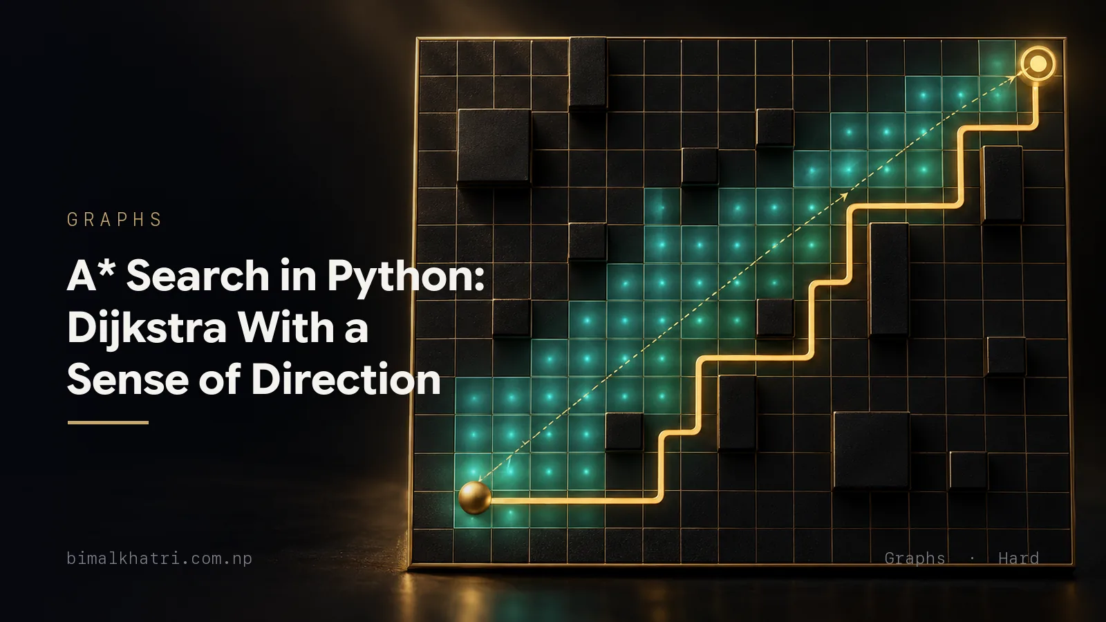
Dijkstra's algorithm has no idea where it is going. It always expands the unfinished node it can reach most cheaply, in every direction at once, so a search from one side of a map to the other spends most of its effort on nodes that point away from the destination. The answer is correct. The work is largely wasted.
A* is Dijkstra plus one addition. Instead of ordering the queue by the cost already spent, order it by the cost already spent plus an estimate of the cost still to come. Nodes that are genuinely nearer the goal rise to the front of the queue, and the search stops fanning out evenly and starts leaning towards the target. On the grid in this post that single change cuts the number of cells the search touches from 59 to 38, and a better tie-break takes it to 24.
The price is that the estimate has to behave itself. If it never overestimates the remaining cost, A* still returns the cheapest path, the guarantee survives intact. If it ever overestimates, A* can finish sooner and return a worse path, silently, with no warning and no crash. What follows is the guarantee, a four-node graph where it is deliberately broken so you can watch the wrong answer come out, and A* counted against Dijkstra on the same grid.
The idea
Every node the search knows about gets three numbers.
- g(n) is the cost of the cheapest route from the start to n that the search has actually found. It is measured, not guessed.
- h(n) is the heuristic: a guess at the cost of getting from n to the goal. It is computed from n and the goal alone, without looking at the graph, which is why it is cheap.
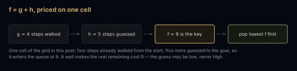
- f(n) = g(n) + h(n) is the search's estimate of the total cost of the best route that passes through n.
A* keeps a priority queue ordered by f, pops the smallest, expands it, and pushes its neighbours with their own f values. That is the whole algorithm.
The two extremes are worth naming, because A* sits exactly between them. Set h(n) = 0 everywhere and f(n) = g(n): the queue is ordered by distance from the start and you have Dijkstra's algorithm, not something like it, the same algorithm, line for line. Drop g(n) instead, order by h alone, and you have greedy best-first search: it charges at the goal, is often very fast, and returns whatever route happened to point the right way. It is not optimal.
A* keeps both terms, and that is what buys the guarantee. But only under a condition.
Admissible: never overestimate
A heuristic is admissible if h(n) is never greater than the true cheapest cost from n to the goal, for every node n. It is allowed to be too low. It is never allowed to be too high.
Here is why that is exactly the right condition. Suppose A* is about to pop the goal with g(goal) = 15, and suppose a cheaper route exists that costs 12. That route starts at a node already expanded and ends at one that is not, so somewhere along it sits a node n still in the queue whose g(n) is already its true best value. Because h never overestimates, h(n) is at most the remaining cost of that route from n, so f(n) = g(n) + h(n) is at most 12. But the goal has f = 15, since h(goal) = 0. A node with f = 12 cannot sit in a min-queue while a node with f = 15 is popped, so the 12-cost route cannot exist.
Turn that over and you can see what breaks it: if h(n) may exceed the real remaining cost, f(n) is pushed above 15 and the good route sinks in the queue. That failure is demonstrated further down.
Consistent: never jump
A stronger property changes what the code is allowed to do. A heuristic is consistent (or monotonic) if h(u) ≤ cost(u, v) + h(v) for every edge from u to v, and h(goal) = 0. It is the triangle inequality applied to the guess: one step cannot cut your estimate of the remaining distance by more than that step costs.
Consistency implies admissibility — chain the inequality along any route to the goal and the terms telescope down to "h(n) ≤ the cost of that route". It also gives what admissibility alone does not: f never decreases along a path, so nodes come out of the queue in non-decreasing f order and the first time a node is popped its g is already final. That is what lets you mark a node finished and never look at it again, exactly as Dijkstra does.
Every grid heuristic below is consistent, which is why grid A* rarely has to think about this. It matters the moment the heuristic is hand-tuned.
Watching it work
The grid is seven rows by ten columns. Movement is up, down, left and right only, and every step costs 1. The # cells are walls, S is the start at row 3, column 0, and G is the goal at row 3, column 9.
The heuristic is Manhattan distance: the steps you would need if the walls were not there. From the start that is 9, since the goal is nine columns right and zero rows away. The true answer is 13, because the wall in column 5 blocks rows 0 to 4 and forces a detour down through row 5.
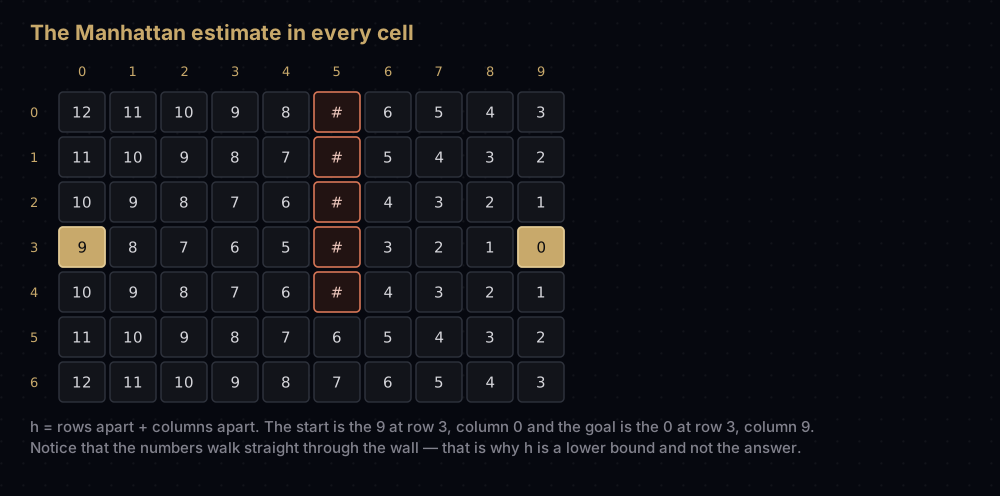
Read that field for a second, because it is the whole trick. The numbers slope smoothly towards the goal and do not notice the wall at all. That is what makes the estimate cheap — two subtractions — and it is also what makes it a lower bound rather than the answer.
Now run the search.
Pop the start. g = 0, h = 9, so f = 9. Its three neighbours go into the queue: row 2 column 0 at f = 1 + 10 = 11, row 4 column 0 at f = 1 + 10 = 11, and row 3 column 1 at f = 1 + 8 = 9.
Pop row 3, column 1, because 9 beats 11. It pushes row 3 column 2 at f = 2 + 7 = 9, and two more cells at f = 11.
The next three pops repeat that. Walking right along row 3 spends one step and saves one step of estimate, so f stays pinned at 9 the whole way. A* drives five cells straight at the goal before anything stops it.
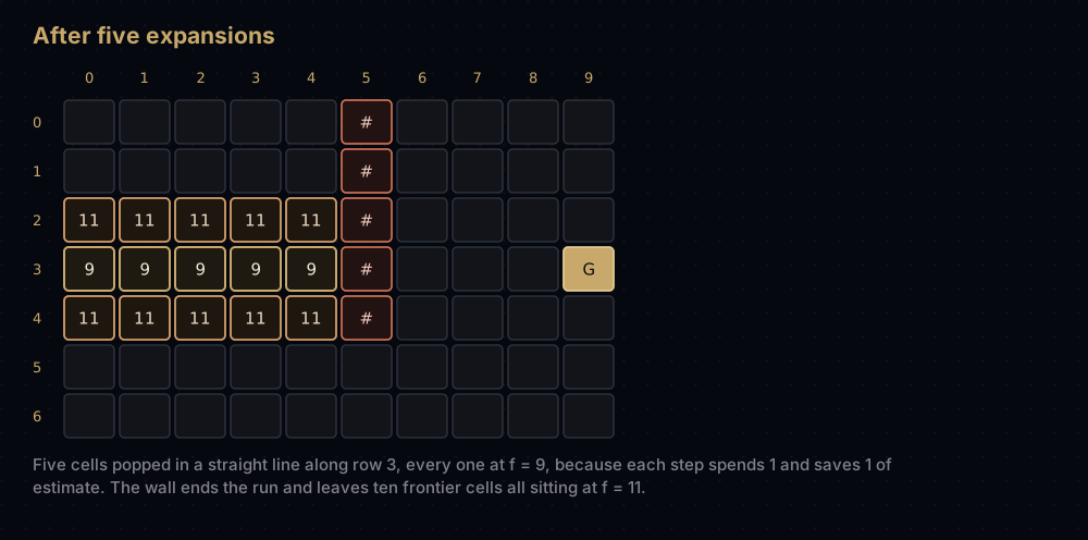
Then the wall. Row 3, column 5 is solid, so expanding row 3 column 4 produces nothing new in that direction. Every entry left in the queue now has f = 11, and there are exactly ten of them, five above row 3 and five below.
That 11 is the search revising its own story: it has proved no route through those cells costs less than 11, so the nine-step dream is dead. It works through the whole f = 11 band, then the f = 13 band, and at 13 it reaches the goal and stops. Nothing in between — one step raises g by 1 and changes h by 1, so f moves by 0 or 2 and its parity never changes. On this grid every f value is odd.
The route it returns is 13 steps: right along row 3 to column 4, down to row 5, right through the gap to column 6, then up to row 3 and right to the goal. Along the way it expanded 38 of the 65 open cells. Dijkstra, on this same grid, expands 59.
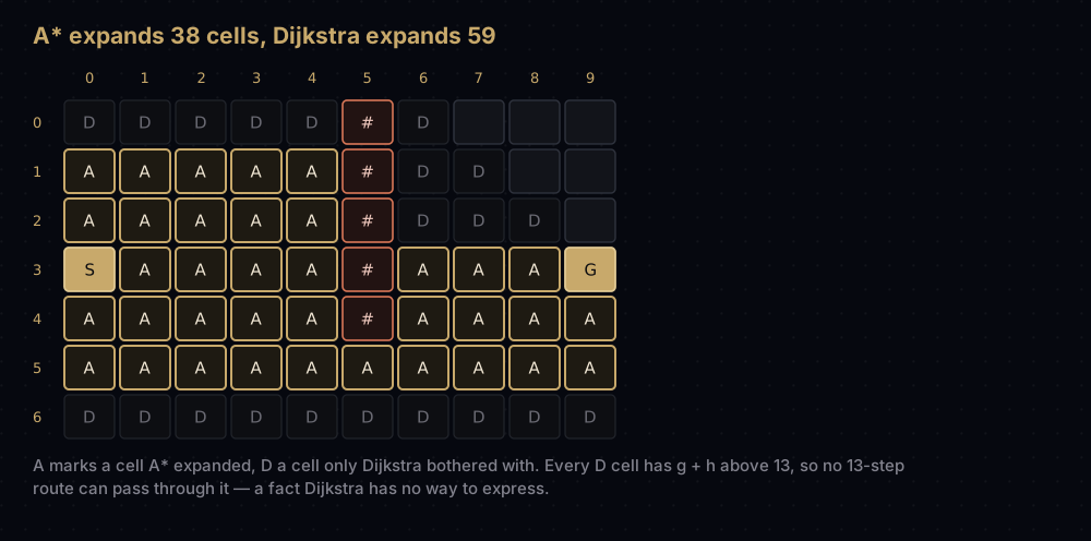
The extra 21 cells sit in the top-left block, the bottom row, and the upper-right pocket behind the wall. Each is a cell A* ruled out without visiting it, because g plus h there already exceeds 13. Row 0, column 0 costs 3 steps to reach and estimates 12 more, so f = 15: no route through it can cost 13. Dijkstra has no way to express that thought, so it walks there anyway.
The code
Start with the grid and the pieces that read it. Keeping the neighbour function separate from the search is what lets the same A* run on a grid, a road network or a puzzle state graph without changes.
from __future__ import annotations

import heapq
import math
from collections.abc import Callable, Iterable
from typing import Any

# '#' is a wall; every other character is walkable. Movement is
# four-directional and every step costs 1.
GRID = [
    ".....#....",
    ".....#....",
    ".....#....",
    "S....#...G",
    ".....#....",
    "..........",
    "..........",
]

START, GOAL = (3, 0), (3, 9)

Cell = tuple[int, int]
# A node is whatever the neighbour function hands back: grid cells here, plain
# strings in the small graphs further down. The search never inspects it.
Node = Any
Neighbours = Callable[[Node], Iterable[tuple[Node, float]]]
Heuristic = Callable[[Node], float]


def grid_moves(grid: list[str]) -> Neighbours:
    """Build the neighbour function for one grid: up, down, left, right, cost 1."""
    rows, cols = len(grid), len(grid[0])

    def moves(cell: Cell) -> Iterable[tuple[Cell, int]]:
        row, col = cell
        for row_step, col_step in ((-1, 0), (1, 0), (0, -1), (0, 1)):
            next_row, next_col = row + row_step, col + col_step
            inside = 0 <= next_row < rows and 0 <= next_col < cols
            if inside and grid[next_row][next_col] != "#":
                yield (next_row, next_col), 1

    return moves


def manhattan(cell: Cell, goal: Cell) -> int:
    """Steps needed on a four-directional grid if nothing were in the way."""
    return abs(cell[0] - goal[0]) + abs(cell[1] - goal[1])


def euclidean(cell: Cell, goal: Cell) -> float:
    """Straight-line distance, which ignores that you cannot move diagonally."""
    return math.hypot(cell[0] - goal[0], cell[1] - goal[1])


def chebyshev(cell: Cell, goal: Cell) -> int:
    """Steps if diagonal moves were allowed and cost the same as straight ones."""
    return max(abs(cell[0] - goal[0]), abs(cell[1] - goal[1]))


def render(grid: list[str], marks: dict[Cell, str]) -> str:
    """Draw the grid, replacing every cell listed in `marks` with its character."""
    return "\n".join(
        "".join(marks.get((row, col), grid[row][col]) for col in range(len(grid[0])))
        for row in range(len(grid))
    )


print(render(GRID, {}))
print(f"{len(GRID)} rows, {len(GRID[0])} columns, "
      f"{sum(row.count('#') for row in GRID)} walls")
print(f"cell (5, 4) -> manhattan {manhattan((5, 4), GOAL)}, "
      f"euclidean {euclidean((5, 4), GOAL):.2f}, "
f"chebyshev {chebyshev((5, 4), GOAL)}").....#....
.....#....
.....#....
S....#...G
.....#....
..........
..........
7 rows, 10 columns, 5 walls
cell (5, 4) -> manhattan 7, euclidean 5.39, chebyshev 5Now the search itself. It is Dijkstra's loop with heuristic(move) added to the key, plus a predecessor table so the route comes back and not just its cost.
def a_star(
    start: Node,
    goal: Node,
    neighbours: Neighbours,
    heuristic: Heuristic,
    tie_break_toward_goal: bool = False,
) -> tuple[dict[Node, Node], float, list[Node]]:
    """Cheapest path from start to goal, with the search steered by heuristic.

    Returns the predecessor table, the cost of the path found, and the nodes in
    the order they were expanded. `heuristic(node)` must never overestimate the
    true remaining cost to the goal, or the path returned can be too expensive.
    """
    best_g = {start: 0}
    came_from = {}
    expanded = []
    # Heap entries are (f, tie-break, g, node). Python compares tuples left to
    # right, so the entry with the smallest f always sits at the root.
    heap = [(heuristic(start), 0, 0, start)]

    while heap:
        _, _, g, node = heapq.heappop(heap)
        if g > best_g[node]:
            continue  # stale: a cheaper route to this node was queued later
        expanded.append(node)
        if node == goal:
            return came_from, g, expanded

        for move, step_cost in neighbours(node):
            candidate = g + step_cost
            if candidate < best_g.get(move, float("inf")):
                best_g[move] = candidate
                came_from[move] = node
                tie = -candidate if tie_break_toward_goal else candidate
                heapq.heappush(
                    heap, (candidate + heuristic(move), tie, candidate, move)
                )

    return came_from, float("inf"), expanded


def reconstruct_path(came_from: dict[Node, Node], start: Node,
                     goal: Node) -> list[Node]:
    """Walk the predecessor chain back from the goal, then reverse it."""
    if goal != start and goal not in came_from:
        return []  # the goal was never reached
    path = [goal]
    while path[-1] != start:
        path.append(came_from[path[-1]])
    path.reverse()
    return path


moves = grid_moves(GRID)
came_from, cost, expanded = a_star(
    START, GOAL, moves, lambda cell: manhattan(cell, GOAL)
)
route = reconstruct_path(came_from, START, GOAL)

print(render(GRID, {cell: "*" for cell in route[1:-1]}))
print(f"cost {cost} over {len(route)} cells, {len(expanded)} cells expanded").....#....
.....#....
.....#....
S****#***G
....*#*...
....***...
..........
cost 13 over 14 cells, 38 cells expandedHow the code maps to the idea
best_g is the g table, one entry per node reached, holding the cheapest route to it found so far. A node missing from the table has not been reached, which is why the comparison uses best_g.get(move, float("inf")): an unseen node loses every comparison, so the first route found always wins.
The heap entry is (f, tie, g, node). Only the first element decides the ordering in the normal case; the rest exist so ties break deliberately rather than by accident, and so a popped entry can report the g it was pushed with.
The stale check is if g > best_g[node]. heapq cannot lower the priority of an entry already in the heap, so an improved node is pushed again and the old entry stays behind carrying a larger g than the table now holds, which is exactly the test. This is the lazy deletion the heapq documentation recommends; rewriting an entry in place would mean maintaining a node-to-index map through every sift.
The goal test is on pop, not on push. When the goal is first generated you have found a route to it; only when it is popped do you know nothing cheaper is left in the queue. Testing on push returns whatever route reached the goal first, which is frequently not the cheapest.
tie_break_toward_goal flips the sign of the second element, so among entries with equal f the one with the larger g wins, and larger g at equal f means smaller h, which means closer to the goal. It changes nothing about correctness and a great deal about speed.
Edge cases fall out of the loop's shape. An unreachable goal drains the heap, the function returns float("inf"), and reconstruct_path returns an empty list. A start that is also the goal pops immediately and returns cost 0 with a one-cell path. Walls need no handling at all: grid_moves never yields them, so they are nodes that do not exist.
Picking a heuristic
On a grid the heuristic is a distance formula, and which one is correct depends entirely on how movement works.
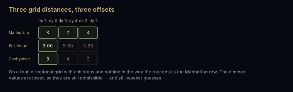
Manhattan, abs(dx) + abs(dy), for four-directional movement. Each step changes exactly one coordinate by one, so an offset of 3 rows and 4 columns takes at least 7 steps. With no walls it is not merely admissible, it is exact, and an exact heuristic is the best one that exists.
Euclidean, hypot(dx, dy), for any-angle movement. Correct when a unit can travel in a straight line at any angle: flying units, navigation meshes, theta*-style path smoothing.
On a four-directional grid Euclidean is still admissible, and it is worth being precise about why: hypot(dx, dy) ≤ abs(dx) + abs(dy) for every offset, and the Manhattan value is itself a lower bound on the real path cost, so the straight line is a lower bound too. But it is a weak one. For an offset of 3 and 4 it reports 5 when the truth is at least 7, so cells off to one side look 2 steps cheaper than they are and get explored anyway. Admissible means correct. It does not mean useful.
Chebyshev, max(abs(dx), abs(dy)), for eight-directional movement where a diagonal costs the same as a straight step. That same offset of 3 and 4 really does take 4 steps. If diagonals cost √2 instead, the right formula is octile distance, max + (√2 − 1) × min.
Run all four against the same grid and they sort exactly by how tight they are:
def no_heuristic(node: Node) -> int:
    """h = 0 is always admissible and always useless: f collapses back to g."""
    return 0


candidates = [
    ("h = 0 (Dijkstra)", no_heuristic),
    ("Chebyshev", lambda cell: chebyshev(cell, GOAL)),
    ("Euclidean", lambda cell: euclidean(cell, GOAL)),
    ("Manhattan", lambda cell: manhattan(cell, GOAL)),
]

seen = {}
for name, heuristic in candidates:
    _, found_cost, cells = a_star(START, GOAL, moves, heuristic)
    seen[name] = cells
    print(f"{name:<17} cost {found_cost:>3}   expanded {len(cells):>3}")

overlay = {cell: "D" for cell in seen["h = 0 (Dijkstra)"]}
overlay.update({cell: "A" for cell in seen["Manhattan"]})
overlay[START], overlay[GOAL] = "S", "G"
print(render(GRID, overlay))h = 0 (Dijkstra) cost 13 expanded 59
Chebyshev cost 13 expanded 51
Euclidean cost 13 expanded 49
Manhattan cost 13 expanded 38
DDDDD#D...
AAAAA#DD..
AAAAA#DDD.
SAAAA#AAAG
AAAAA#AAAA
AAAAAAAAAA
DDDDDDDDDDEvery one returns 13, because every one is admissible. What changes is the bill. The map below the table is the overlay from the walkthrough, printed by the code that produced it: A for cells Manhattan A* expanded, D for cells only Dijkstra bothered with.
The rule generalises, but only for consistent heuristics. If two heuristics are both consistent and one is never smaller than the other, the larger expands a subset of the smaller one's nodes, apart from the nodes whose f exactly equals the optimal cost, where tie-breaking decides. Admissible on its own is not enough: an inconsistent heuristic lets the search re-expand nodes, and then the tighter guess can do more work, not less. On the four-node graph in "Admissible is not the same as consistent" below, h = 0 expands four nodes and the larger admissible heuristic expands five.
Ties are where the rest of the win is
Ten cells sat at f = 11 in the walkthrough, and nothing in plain A* says which to take first. Taking them in an arbitrary order sweeps the whole equal-f band like a breadth-first search before committing to any direction. Preferring the entry with the larger g drives one branch to its conclusion instead.
def room(rows: int, cols: int, wall_col: int, gap: int) -> list[str]:
    """An open room split by one vertical wall that stops `gap` rows short."""
    return ["".join("#" if col == wall_col and row < rows - gap else "."
                    for col in range(cols))
            for row in range(rows)]


def corridors(rows: int, cols: int) -> list[str]:
    """A serpentine maze: vertical walls whose gap alternates top and bottom."""
    return ["".join("#" if col % 6 == 5 and ((row < rows - 3) if (col // 6) % 2 == 0
                                             else (row > 2)) else "."
                    for col in range(cols))
            for row in range(rows)]


def compare(label: str, grid: list[str], start: Cell, goal: Cell) -> None:
    """Print how many cells Dijkstra and A* expand on the same grid."""
    neighbours = grid_moves(grid)

    def heuristic(cell: Cell) -> int:
        return manhattan(cell, goal)

    _, path_cost, dijkstra_cells = a_star(start, goal, neighbours, no_heuristic)
    _, _, plain = a_star(start, goal, neighbours, heuristic)
    _, _, tuned = a_star(start, goal, neighbours, heuristic,
                         tie_break_toward_goal=True)
    open_cells = sum(1 for row in grid for square in row if square != "#")
    print(f"{label:<18} cost {path_cost:>4}  open {open_cells:>4}  "
          f"Dijkstra {len(dijkstra_cells):>4}  A* {len(plain):>4}  "
          f"A* tie-broken {len(tuned):>4}")


compare("10 x 7 one wall", GRID, START, GOAL)
compare("31 x 21 one wall", room(21, 31, 15, 3), (10, 0), (10, 30))
compare("31 x 21 corridors", corridors(21, 31), (0, 0), (20, 30))10 x 7 one wall cost 13 open 65 Dijkstra 59 A* 38 A* tie-broken 24
31 x 21 one wall cost 46 open 633 Dijkstra 578 A* 391 A* tie-broken 251
31 x 21 corridors cost 114 open 561 Dijkstra 545 A* 521 A* tie-broken 441The third line is the honest one. In a serpentine maze the Manhattan estimate is systematically wrong — the goal is a few cells away in a straight line and a hundred steps away through the corridors — so A* saves 4% and nothing more. A heuristic helps only to the extent that it correlates with reality. When it does not, A* is Dijkstra plus a function call per node.
What an inadmissible heuristic costs you
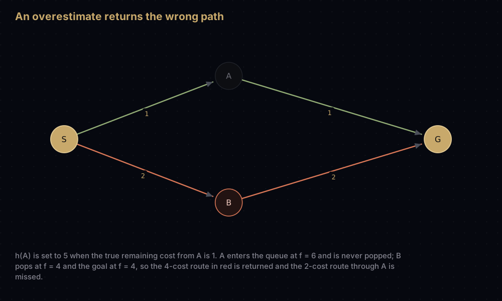
Four nodes. S reaches A for 1 and B for 2; A reaches the goal for 1, B reaches it for 2. The cheapest route is S to A to G, total 2. Now lie about A: set h(A) = 5 when the truth is 1, and leave everything else honest.
DETOUR = {
    "S": [("A", 1), ("B", 2)],
    "A": [("G", 1)],
    "B": [("G", 2)],
    "G": [],
}

honest = {"S": 2, "A": 1, "B": 2, "G": 0}
inflated = {"S": 2, "A": 5, "B": 2, "G": 0}

for name, table in [("admissible", honest), ("inadmissible", inflated)]:
    trail, trail_cost, _ = a_star(
        "S", "G", lambda node: DETOUR[node], lambda node: table[node]
    )
    print(f"{name:<13} h(A) = {table['A']}   cost {trail_cost}   "
f"{' -> '.join(reconstruct_path(trail, 'S', 'G'))}")admissible h(A) = 1 cost 2 S -> A -> G
inadmissible h(A) = 5 cost 4 S -> B -> GTrace the second run and the mechanism is plain. S pops and queues both neighbours: A at f = 1 + 5 = 6, B at f = 2 + 2 = 4. B is smaller, so B pops and queues the goal at f = 4 + 0 = 4. The goal is now the smallest entry, so it pops and the search returns, while A, the first step of the optimal route, sits in the queue at 6, never examined. Nothing crashes. A path is returned. It costs twice what it should.
This is the same class of failure as running Dijkstra on negative edges: plausible output, no error, visible only on the inputs where it matters. If you hand-tune a heuristic, test it by comparing against Dijkstra on a few hundred generated graphs and asserting equal costs.
One case breaks admissibility on purpose. Weighted A* uses f = g + w × h with w above 1, exploring far fewer nodes and returning a path guaranteed to cost at most w times the optimum. Games and planners use it when a route 10% long found in a millisecond beats a perfect route found in twenty. Do it deliberately, with a known w, and quote the bound.
Admissible is not the same as consistent
Textbook A* usually keeps a closed set: once a node is expanded, never touch it again. That is a genuine saving, and it is valid only if the heuristic is consistent.
The graph: S reaches A for 4 and B for 1, B reaches A for 1, A reaches the goal for 5. The best route is S to B to A to G, total 7. Set h(S) = 0, h(A) = 0, h(B) = 4, h(G) = 0. Every value is at or below the true remaining cost, so this is admissible. But the edge B to A costs 1 while h drops from 4 to 0, so h(B) ≤ cost(B, A) + h(A) fails: not consistent.
DIVERSION = {
    "S": [("A", 4), ("B", 1)],
    "A": [("G", 5)],
    "B": [("A", 1)],
    "G": [],
}

# Admissible (nothing here exceeds the true remaining cost) but not consistent:
# h(B) = 4 while the single step B -> A costs 1 and h(A) = 0.
inconsistent = {"S": 0, "A": 0, "B": 4, "G": 0}


def a_star_closed(start: Node, goal: Node, neighbours: Neighbours,
                  heuristic: Heuristic) -> tuple[dict[Node, Node], float]:
    """A* that never revisits an expanded node. Safe only if h is consistent."""
    best_g = {start: 0}
    came_from = {}
    closed = set()
    heap = [(heuristic(start), 0, start)]

    while heap:
        _, g, node = heapq.heappop(heap)
        if node in closed:
            continue
        closed.add(node)
        if node == goal:
            return came_from, g
        for move, step_cost in neighbours(node):
            if move in closed:
                continue  # assumed final, and that assumption is the bug
            candidate = g + step_cost
            if candidate < best_g.get(move, float("inf")):
                best_g[move] = candidate
                came_from[move] = node
                heapq.heappush(heap, (candidate + heuristic(move), candidate, move))

    return came_from, float("inf")


open_trail, open_cost, open_expanded = a_star(
    "S", "G", lambda node: DIVERSION[node], lambda node: inconsistent[node]
)
closed_trail, closed_cost = a_star_closed(
    "S", "G", lambda node: DIVERSION[node], lambda node: inconsistent[node]
)
print(f"re-expanding   cost {open_cost}   "
      f"{' -> '.join(reconstruct_path(open_trail, 'S', 'G'))}   "
      f"expanded {', '.join(open_expanded)}")
print(f"closed set     cost {closed_cost}   "
f"{' -> '.join(reconstruct_path(closed_trail, 'S', 'G'))}")re-expanding cost 7 S -> B -> A -> G expanded S, A, B, A, G
closed set cost 9 S -> A -> GA is popped early at g = 4, because f = 4 + 0 = 4 beats B's f = 1 + 4 = 5. Later B is popped and offers A a route costing 2. The version at the top of this post accepts it, pushes A again, and expands A a second time. That is the repeated A in the expansion list, and it is what buys the correct answer of 7. The closed-set version refuses to look at A again and reports 9.
Both fixes are legitimate. Use a consistent heuristic and keep the closed set, or allow re-expansion as the code here does. Every grid heuristic in this post is consistent, so on a grid the closed set is free.
Complexity
Time is Dijkstra's, because the worst case is Dijkstra. Assume a consistent heuristic, so each node is expanded at most once. Expanding a node scans its outgoing edges exactly once, so across the whole run there are at most E edge scans. Each scan pushes at most one heap entry, so the heap takes at most E + 1 entries and gives back at most E + 1. Each push and pop sifts along one root-to-leaf path of a binary heap holding at most E + 1 items, which is O(log E) comparisons. Since E is at most V², log E is at most 2 log V, and constants vanish. Add O(V) for the tables and the total is O((V + E) log V). On a four-directional grid each cell has at most 4 neighbours, so E ≤ 4V and that collapses to O(V log V).
The bound that actually predicts the runtime is not asymptotic. With a consistent heuristic and an optimal path costing C, A* expands every reachable node whose f value is below C, no node whose f value is above C, and some of the nodes exactly equal to C, decided by tie-breaking. That single sentence explains every number in this post:
| Grid | Open cells | Dijkstra | A*, plain ties | A*, ties toward the goal |
|---|---|---|---|---|
| 10 × 7, one wall | 65 | 59 | 38 | 24 |
| 31 × 21, one wall | 633 | 578 | 391 | 251 |
| 31 × 21, corridors | 561 | 545 | 521 | 441 |
Because f(n) = g(n) + h(n), raising h at a node raises its f, so it can only push that node out of the "below C" set, never into it. That is the formal version of "a tighter heuristic explores less". With h = 0 the set is every node within C of the start, which is Dijkstra. With a perfect heuristic and good tie-breaking, the set is the optimal path itself.
Space is O(V) for the tables plus O(E) for the heap, and that, not the time bound, is A*'s real practical limit. Both best_g and came_from hold one entry per node reached, and a search over a large state space — the 15-puzzle has about 10 trillion — runs out of memory long before it runs out of patience. That is what IDA* exists for: it re-runs a depth-first search with an increasing f cutoff and keeps only the current path, trading repeated work for O(depth) space.
Two things can make it worse. An inconsistent heuristic plus re-expansion can revisit nodes many times over; there are constructed graphs where the expansion count grows exponentially in the number of nodes. And the heuristic is charged once per generated node, so an estimate that costs more than the search it saves is a net loss. Manhattan is two subtractions, which is the point.
When to use it, and when not to
Use it when you have one specific target, a heuristic that is cheap and admissible, and a graph big enough that the saving matters. That describes almost all single-unit pathfinding.
Do not use it when you have no meaningful estimate of the remaining cost. h = 0 is admissible, so A* still works, but it is Dijkstra with an extra function call per node generated. Write Dijkstra.
Do not use it when every edge costs the same. Breadth-first search finds that shortest path in O(V + E) with a collections.deque and no heap, no heuristic and no arithmetic.
Do not use it when many agents head for the same destination. One Dijkstra run outward from the goal gives every node its exact distance and each agent then walks downhill: one search instead of a hundred. Game engines call the result a flow field.
Do not use it when any edge weight can be negative. A* inherits that limitation exactly: once a later edge can reduce a total, popping the smallest f proves nothing. Use Bellman-Ford.
Do not use it when the graph is fixed and you serve millions of queries against it. Continental road routing precomputes contraction hierarchies offline and answers in microseconds against the compressed graph. A* is the correctness baseline those are measured against.
Where it shows up in the real world
Game pathfinding. This is A*'s home ground. Recast and Detour, the open-source navigation-mesh toolkit many shipped games build on, runs A* over navmesh polygons in dtNavMeshQuery::findPath. Unity's NavMeshAgent and Unreal Engine's navigation system both do the same over a generated navmesh, with a Euclidean heuristic.
Robotics motion planning. ROS navigation stacks run A* and Dijkstra variants over an occupancy-grid costmap as the global planner, leaving a local controller to handle obstacles that appear after the plan is made. For car-like vehicles that cannot turn on the spot, Hybrid A* searches a continuous space of position and heading; it was developed for Stanford's DARPA Urban Challenge entry and is standard in autonomous-parking work.
Puzzle and planning search. The 15-puzzle is the canonical A* benchmark, with the sum of every tile's Manhattan distance from its target as the heuristic: admissible because one move relocates exactly one tile by one square.
Route planners, as a foundation. Bidirectional A* over a road graph is a real production technique, and the landmark-based ALT heuristic (precompute exact distances to a few dozen landmark nodes, then apply the triangle inequality) gives a far tighter estimate than straight-line distance. Modern engines add contraction hierarchies on top, but the search underneath is still this loop.
In Python, there is no A* in the standard library; heapq gives you the queue. networkx.astar_path takes a graph, a source, a target and a heuristic function, and is the fastest way to sanity-check an implementation.
Common mistakes
Testing for the goal when you push instead of when you pop. The single most common A* bug. Returning as soon as the goal is generated returns the first route found, not the cheapest, and the code looks perfectly correct because it does return a valid path.
A heuristic in the wrong units. If every step costs 10 and your heuristic returns a count of steps, h is ten times too small and A* degenerates into Dijkstra. If steps cost 1 and your heuristic returns metres, h is far too large, admissibility is gone and the paths are wrong. Multiply the estimate by the cost of one unit of distance.
Squared Euclidean distance. Skipping the square root is tempting because it is faster and the ordering looks the same. It is not admissible: for an offset of 3 rows and 4 columns it returns 25 where the true four-directional cost is 7, so it overestimates wildly and returns bad paths.
Keeping a closed set with a hand-tuned heuristic. Fine for the standard grid formulas, which are all consistent. Not fine for an estimate you invented, as the nine-versus-seven example above shows.
Ignoring ties. A correct A* that breaks ties arbitrarily expands about half again as many nodes as one that breaks them toward the goal: 38 against 24 on the small grid here, 391 against 251 on the larger one. It is a one-line change.
Making the heuristic expensive. A* is only ahead of Dijkstra when h is cheap, because it is charged once for every node generated. Manhattan is two subtractions and an addition. If your estimate needs a lookup or a square root you cannot avoid, measure whether the expansions you save actually pay for it.
Practice
- Print the
expandedlist thata_staralready returns and confirm the first five cells on the example grid are the straight run along row 3. - Make the grid eight-directional by adding the four diagonal moves at cost 1, switch the heuristic to Chebyshev, and check that the path cost drops from 13.
- Give some cells a movement cost of 5 instead of 1 (mud, or water) and confirm A* routes around them, then confirm that leaving the heuristic unscaled still returns the correct path but expands many more cells.
- Implement greedy best-first search by using h alone as the priority, and find a grid where it returns a path longer than 13.
- Write a checker that generates 200 random grids with a fixed seed, runs A* and Dijkstra on each, and asserts the costs match: then break it deliberately by multiplying the heuristic by 2 and watch which grids fail.
Summary
A* is Dijkstra with a second term in the priority. That term, h(n), is a guess at how much is left, and everything about the algorithm follows from one rule: the guess must never be too high. Keep it admissible and the shortest path is still guaranteed. Make it tighter and the search touches fewer nodes, because A* expands every node whose g + h falls below the optimal cost and only some of those that equal it. Set it to zero and you are back to Dijkstra, which is the point: A* is not a different algorithm, it is the same one given a sense of direction.
| Difficulty | Hard |
| Time | O((V + E) log V) — with a consistent heuristic each node expands once, each edge pushes at most one heap entry, and each heap operation costs O(log E) |
| Nodes expanded | Every node with g + h below the optimal cost, plus some of those equal to it |
| Space | O(V) for the g and predecessor tables plus up to O(E) heap entries — memory is the practical limit |
| Graph type | Directed or undirected, weighted, non-negative weights only |
| Returns optimal path | Yes, if the heuristic never overestimates |
| Re-expands nodes | No if the heuristic is consistent; otherwise yes, unless you keep a closed set and accept wrong answers |
| With h = 0 | Exactly Dijkstra's algorithm |
| Handles negative weights | No — same failure as Dijkstra; use Bellman-Ford |
| Use it when | One target, and a cheap estimate of the distance to it that never overestimates |
| Avoid it when | No useful heuristic (Dijkstra), uniform edges (BFS), many targets (one reverse Dijkstra), negative weights (Bellman-Ford), tight memory (IDA*) |
| Real-world use | Navmesh pathfinding in Recast/Detour, Unity and Unreal; robot global planners; Hybrid A* for vehicles; 15-puzzle search |
| Python equivalent | None in the standard library; heapq supplies the queue, networkx.astar_path if a dependency is acceptable |
Keep reading
- Dijkstra's Algorithm — the algorithm A* generalises, and the invariant that both of them rest on.
- Breadth-First Search — what to run when every edge costs the same and a heuristic buys you nothing.
- Heaps and Priority Queues — where the log in every bound above comes from, sift by sift.
- Graphs in Python — adjacency lists, matrices, and how to feed a grid to a graph algorithm.
- Greedy Algorithms — why taking the locally best option works for A*'s queue and fails for its cousin, greedy best-first search.


