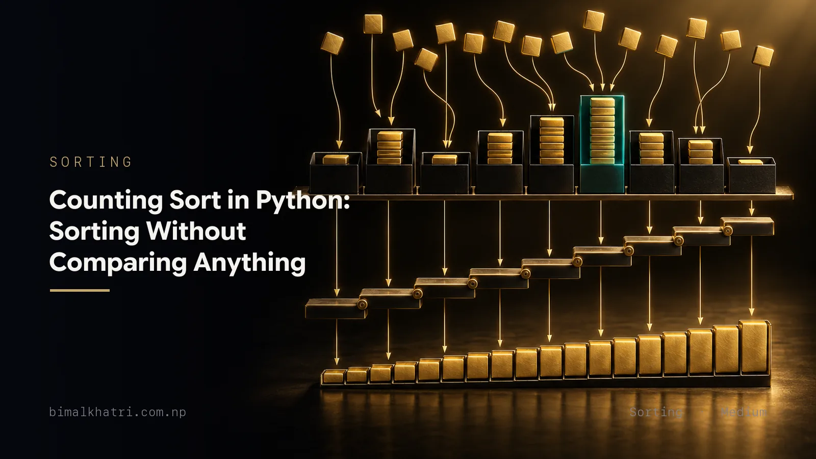
Every sorting algorithm in this series so far asks the same question over and over: is this item bigger than that one? Bubble sort asks it about neighbours, merge sort asks it about the fronts of two runs, quick sort asks it about a pivot. Counting sort never asks it once. It reads a value, uses that value as an index into an array of counters, adds one, and moves on. Then it reads the counters back. There is not a single comparison anywhere in the algorithm.
That is not a presentational trick. There is a proof (the decision-tree argument, worked through below) that no algorithm sorting by comparison can do better than O(n log n) comparisons in the worst case. It is a hard floor, and merge sort sits exactly on it. Counting sort runs in O(n + k), where k is the size of the range the keys are drawn from, which is linear whenever k is proportional to n. It gets there by stepping outside the model the proof applies to.
The price is worth stating before the good part. You must know the range of the keys, and you allocate one counter for every possible value in that range, whether or not any item uses it. Sort a thousand arbitrary 32-bit integers this way and you will ask Python for 4.29 billion counters — about 32 GB — to order a thousand numbers that sorted() handles in roughly ten thousand comparisons. Counting sort is extraordinary inside a narrow lane and useless outside it, and knowing exactly where that lane ends is most of the value in learning it.
The idea
Suppose every value in your list is an integer between 0 and 5. You do not need to compare anything to sort it. You only need to know how many 0s it contains, how many 1s, and so on up to 5. Once you have the tally, the sorted output writes itself: print every 0, then every 1, then every 2, and you are done.
So make an array of six counters, all zero. Walk the list once and, for each value, add one to the counter at that index. One pass, one increment per item, no comparisons.
For bare integers that really is the whole algorithm, in six lines of code. But it quietly throws something away. In real work you rarely sort naked numbers. You sort records by an integer field: support tickets by priority, pixels by brightness, players by score. Rebuilding the output from a tally produces fresh copies of the key and loses everything attached to it. Two tickets at priority 3 are not interchangeable; they have different bodies.
So the usable version moves the original items instead, and to do that it must know which output slot each item belongs in before it moves anything. That takes one extra step, and it is the step worth learning:
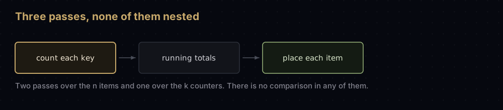
- Count. For each key value, how many items carry it. One pass over n items.
- Prefix sums. Turn the counts into starting positions. One pass over the k counters.
- Place. Walk the input and drop each item into the next free slot for its key. One pass over n items.
Phase 2 rests on a single observation. If four items have a key smaller than 3, the first 3 must land in output slot 4: slots 0 to 3 are already spoken for and there is nowhere else for it to go. And "how many items have a key smaller than 3" is just the sum of the counters below index 3. A running total over the count array therefore converts counts into addresses. That running total is a prefix sum, one of the most reusable ideas in this series.
Phase 3 then hands out each key's slots in order: the first item with key 3 takes slot 4, the next takes slot 5, the next takes slot 6. Walk the input from left to right and ties come out in the order they went in. That property is stability, and here it is not a nicety. It is the reason the algorithm is useful at all, as the radix sort section shows.
Watching it work
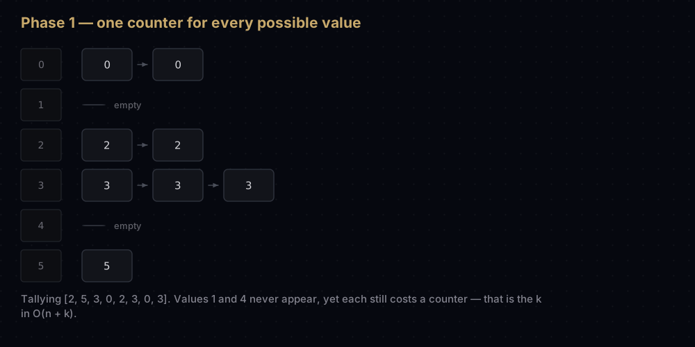
Sort [2, 5, 3, 0, 2, 3, 0, 3]. Eight items, keys drawn from 0 to 5, so n is 8 and k is 6.
Phase 1: count
Walk the list and tally. Two 0s, no 1s, two 2s, three 3s, no 4s, one 5. The counts sum to 8, which they must: every item is counted exactly once.
Phase 2: prefix sums
Now convert those counts into starting positions. Sweep left to right with a running total, writing the total before adding the current count:
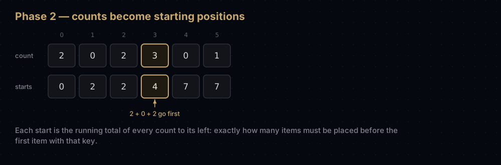
Read the second row as a list of addresses. The first 0 goes in slot 0, the first 2 in slot 2, the first 3 in slot 4, the first 5 in slot 7. Values 1 and 4 never appear, so their starting positions match the next value's: they own an empty stretch of output, which is exactly right. Note that this sweep runs over the counters, not the items: it costs k steps, not n.
Phase 3: place
Walk the input from left to right. For each item, look up the starting position for its key, write the item there, then bump that position by one so the next item with the same key lands beside it.
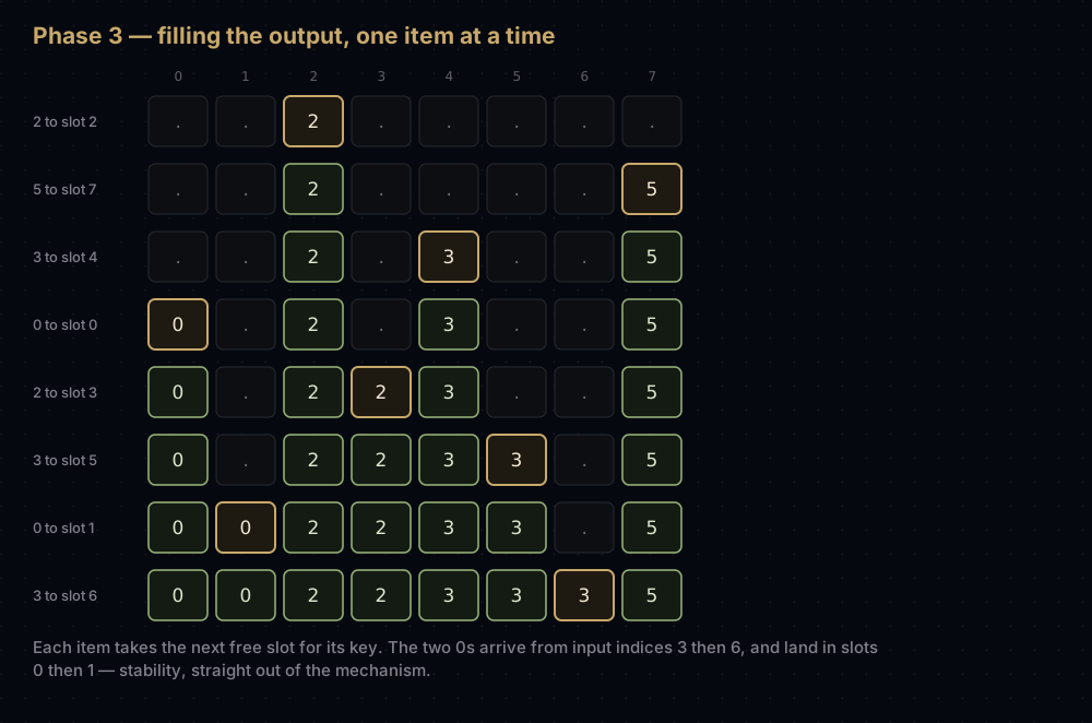
Follow the two 0s, because they show the stability. They sit at input indices 3 and 6. The first one processed takes slot 0 and pushes the cursor to 1, so the second takes slot 1; their relative order survived. That is not luck, it follows from scanning the input forwards and handing out slots forwards. The three 3s do the same, taking slots 4, 5 and 6 in input order. Eight writes, eight cursor bumps, no comparisons, and a final output of [0, 0, 2, 2, 3, 3, 3, 5].
The code
Start with the crude version, because for plain integers it is genuinely all you need and it makes the counting phase obvious.
def counting_sort_simple(values: list[int]) -> list[int]:
    """Sort non-negative integers by tallying each value, then reading the tally back.

    Only safe for bare integers: it rebuilds the equal values from a count
    rather than moving the originals, so anything attached to them is lost.
    """
    if not values:
        return []

    counts = [0] * (max(values) + 1)
    for value in values:
        counts[value] += 1

    result: list[int] = []
    for value, count in enumerate(counts):
        result.extend([value] * count)
    return result


print(counting_sort_simple([2, 5, 3, 0, 2, 3, 0, 3]))
print(counting_sort_simple([]))
print(counting_sort_simple([7]))[0, 0, 2, 2, 3, 3, 3, 5]
[]
[7]Correct, linear, and unusable the moment the things you are sorting carry any data besides the key. Here is the real one, with the prefix-sum phase and a key function so it can sort records.
from typing import Any, Callable


def counting_sort(items: list[Any],
                  key: Callable[[Any], int] = lambda item: item) -> list[Any]:
    """Sort items by an integer key in O(n + k), keeping ties in input order.

    key(item) must return an int. The counters span the smallest key seen to
    the largest, so negative keys work and k is the range actually used rather
    than the whole integer type.
    """
    if not items:
        return []

    keys = [key(item) for item in items]
    lowest, highest = min(keys), max(keys)
    span = highest - lowest + 1

    # Phase 1 - how many items carry each key.
    counts = [0] * span
    for value in keys:
        counts[value - lowest] += 1

    # Phase 2 - starting positions. starts[i] is the first output slot owned by
    # that key, which is exactly the number of items with a smaller key.
    starts = [0] * span
    running = 0
    for index, count in enumerate(counts):
        starts[index] = running
        running += count

    # Phase 3 - walk the input forwards and drop each item into the next free
    # slot for its key. Forwards plus the increment is what keeps ties in order.
    output: list[Any] = [None] * len(items)
    for item, value in zip(items, keys):
        slot = value - lowest
        output[starts[slot]] = item
        starts[slot] += 1

    return output


print(counting_sort([2, 5, 3, 0, 2, 3, 0, 3]))
print(counting_sort([-3, 4, -1, 0, -3]))
print(counting_sort([]))
print(counting_sort([9, 9, 9]))[0, 0, 2, 2, 3, 3, 3, 5]
[-3, -3, -1, 0, 4]
[]
[9, 9, 9]Because it moves the original objects rather than rebuilding them, it sorts records and keeps ties in input order:
tickets = [
    ("ana", 3), ("bo", 1), ("cy", 3), ("dee", 0), ("eli", 1), ("fin", 3),
]
for name, priority in counting_sort(tickets, key=lambda row: row[1]):
print(f"{name:<4} {priority}")dee 0
bo 1
eli 1
ana 3
cy 3
fin 3Three tickets sit at priority 3 and they come out as ana, cy, fin: the order they arrived in. That is a first-in-first-out queue within each priority level, which is usually what you want and never something you get for free from quick sort or heap sort.
To confirm the walkthrough above was not wishful thinking, here is the same algorithm printing every intermediate state:
def counting_sort_traced(values: list[int]) -> list[int]:
    """Counting sort that prints the counts, the starting positions and every write."""
    lowest = min(values)
    counts = [0] * (max(values) - lowest + 1)
    for value in values:
        counts[value - lowest] += 1
    print(f"counts  {counts}")

    starts, running = [0] * len(counts), 0
    for index, count in enumerate(counts):
        starts[index] = running
        running += count
    print(f"starts  {starts}")

    output: list[int | None] = [None] * len(values)
    for value in values:
        slot = value - lowest
        position = starts[slot]
        output[position] = value
        starts[slot] += 1
        picture = " ".join("." if cell is None else str(cell) for cell in output)
        print(f"{value} -> slot {position}   {picture}")

    return [cell for cell in output if cell is not None]


counting_sort_traced([2, 5, 3, 0, 2, 3, 0, 3])counts [2, 0, 2, 3, 0, 1]
starts [0, 2, 2, 4, 7, 7]
2 -> slot 2 . . 2 . . . . .
5 -> slot 7 . . 2 . . . . 5
3 -> slot 4 . . 2 . 3 . . 5
0 -> slot 0 0 . 2 . 3 . . 5
2 -> slot 3 0 . 2 2 3 . . 5
3 -> slot 5 0 . 2 2 3 3 . 5
0 -> slot 1 0 0 2 2 3 3 . 5
3 -> slot 6 0 0 2 2 3 3 3 5Every line matches the diagram, including the order the slots are claimed in. Notice how scattered the writes are: slot 2, then 7, then 4, then 0. Counting sort jumps around the output array, which is why its cache behaviour is worse than its instruction count suggests.
How the code maps to the idea
Keys are computed once, into their own list. Three passes run over the items (the min/max sweep, phase 1 and phase 3), so calling key(item) in each of them would triple the cost of the most expensive operation in the function. Computing keys up front costs one list of n integers and makes every later use a plain index.
Subtracting lowest is what makes negative keys work. In Python, counts[-3] += 1 does not raise: it silently increments the third counter from the end of the list, producing a wrong answer with no error at all. Offsetting every key by the minimum turns any range into one starting at 0. It also shrinks k: sorting years between 1990 and 2026 needs 37 counters, not 2,027.
Three loops, none of them nested. Loop one runs n times, loop two runs k times, loop three runs n times. That flat structure is the O(n + k) bound; you can read it off the indentation. No branch anywhere depends on how the data is arranged, which is why counting sort has no best or worst case.
The output list is pre-allocated to exactly len(items), because the counts sum to n and you know the final length before writing anything. No appending, no resizing.
Forward scan plus starts[slot] += 1 is the stability. The two work as a pair: scanning forwards places earlier items first, and incrementing gives each one the lowest still-free slot for its key. Reverse either half and equal items come out backwards. The equally common CLRS variant builds inclusive prefix sums — each entry counting the items with a key less than or equal to that key — then walks the input backwards, decrementing. That is stable too, for the mirror-image reason. Mixing the two conventions is not.
The edge cases fall out of the arithmetic, with one exception: an empty list needs the explicit if not items guard, because min([]) raises ValueError. Everything else is free. A single item gives span == 1; a list of identical values gives span == 1 and one counter holding them all; a range with holes in it gives counters that stay at zero and starting positions that repeat.
Complexity
Counting the work
Add up everything the function does.
- Building
keystouches each item once: n steps. min(keys)andmax(keys)each sweep that list to find the span: 2n steps.- Zeroing the two k-slot arrays,
countsandstarts: 2k steps. - Phase 1 does one increment per item: n steps.
- Phase 2 does one addition per counter: k steps.
- Filling the output list with
None: n steps. - Phase 3 does one lookup, one write and one increment per item: n steps.
Total: 6n + 3k constant-time operations. Big O discards the constants and leaves O(n + k).
No loop contains a data-dependent branch, so the best, average and worst cases are all Θ(n + k). Already-sorted input costs the same as reversed input costs the same as random input. Counting sort is not adaptive, and it cannot be given a bad day.
Space is O(n + k): two k-slot arrays, n output slots and n keys. The crude version at the top of the code section is no cheaper. It skips the starts array and the key list, but it still allocates k counters and still builds an n-element result, so it is O(n + k) as well. What it saves is code, not memory, and it pays for that saving by rebuilding equal values from a tally instead of moving the originals, which is why it cannot sort records at all.
The n + k is a sum, not a product, and that matters. If k is 100 and n is 10,000,000, the k term vanishes. If k is 10,000,000 and n is 100, the n term vanishes and you have spent ten million steps sorting a hundred items.
Why no comparison sort can do this
Counting sort beats O(n log n), and there is a theorem saying that is impossible. Both statements are true, and reconciling them is the most useful idea here.
Take any algorithm whose only way of learning about the data is to ask "is a smaller than b?". Every such question has two answers, so a run of the algorithm is a walk down a binary tree: the root is the first comparison, each branch is one answer, each leaf a finished arrangement. Here is the entire tree for three items:
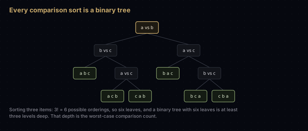
Two facts about that tree finish the argument.
It must have at least n! leaves. With n distinct items there are n! possible input orderings, each needing a different sequence of moves to sort. If two orderings ended at the same leaf, the algorithm would make identical moves on both, and at most one of those results can be sorted. Three items, six leaves.
A binary tree of height h has at most 2ʰ leaves, since each level at most doubles the node count. So 2ʰ ≥ n!, which means h ≥ log₂(n!).
The height of the tree is the number of comparisons along the longest path, the worst case. So every comparison sort needs at least log₂(n!) comparisons on some input. Stirling's approximation turns log₂(n!) into n log₂ n − 1.44n + O(log n), which is Ω(n log n). Merge sort's guaranteed n log₂ n hits that floor almost exactly.
The floor is not abstract. Here it is beside the work counting sort does when k equals n:
import math

print(f"{'n':>9}  {'log2(n!)':>14}  {'n + k, k = n':>13}")
for n in [10, 100, 1_000, 1_000_000]:
    lower_bound = math.lgamma(n + 1) / math.log(2)
print(f"{n:>9,} {lower_bound:>14,.0f} {2 * n:>13,}") n log2(n!) n + k, k = n
10 22 20
100 525 200
1,000 8,529 2,000
1,000,000 18,488,885 2,000,000At a thousand items, no comparison sort in existence can guarantee fewer than 8,529 comparisons, while counting sort finishes in about 2,000 steps. At a million the gap is nine-fold and growing, because one column grows like n and the other like n log n.
So how does counting sort get under a proven floor? It never makes a comparison, so it is not in the tree. Indexing counts[value] is not a two-way question but a k-way jump, and one of those distinguishes between k possibilities rather than 2. The proof bounds algorithms that extract one bit of information at a time; counting sort extracts log₂ k bits per operation by treating the key as an address.
The bill arrives as an assumption: the keys must be integers in a known, bounded range, dense enough that one slot per possible value is affordable. Comparison sorts need none of that: they sort strings, floats, tuples, dates and anything else with an ordering. The lower bound is the price of that generality, and counting sort's memory is the price of escaping it.
The k problem
k is the range of the keys, not the number of distinct keys, and that distinction destroys more counting-sort implementations than anything else. The list [1, 5, 1000000] has three items and three distinct values, but k is 1,000,000. You allocate a million counters, set three of them to 1, and sweep all million in phase 2 to sort three numbers.
The memory is the hard wall. A CPython list holds one 8-byte pointer per slot, so the count array costs 8k bytes at minimum:
def human_bytes(count: int) -> str:
    """Format a byte count with the largest unit that keeps it above 1."""
    size = float(count)
    for unit in ["B", "KB", "MB", "GB", "TB", "PB", "EB"]:
        if size < 1024:
            return f"{size:.1f} {unit}"
        size /= 1024
    return f"{size:.1f} ZB"


for label, k in [
    ("exam scores, 0-100", 101),
    ("one byte, 0-255", 256),
    ("seconds in a year", 60 * 60 * 24 * 365),
    ("32-bit signed ints", 2 ** 32),
    ("64-bit signed ints", 2 ** 64),
]:
print(f"{label:<20} k = {k:>26,} counters = {human_bytes(k * 8):>9}")exam scores, 0-100 k = 101 counters = 808.0 B
one byte, 0-255 k = 256 counters = 2.0 KB
seconds in a year k = 31,536,000 counters = 240.6 MB
32-bit signed ints k = 4,294,967,296 counters = 32.0 GB
64-bit signed ints k = 18,446,744,073,709,551,616 counters = 128.0 EBThe concrete failure promised in the opening is the fourth row. Sorting a thousand user IDs spread across the full 32-bit range needs a 32 GB array of counters and 4.29 billion steps to sweep it in phase 2, and exactly a thousand of those counters end up nonzero. sorted() does the same job in under ten thousand comparisons and no allocation worth measuring. The bottom row is not merely slow: 128 exabytes exceeds the storage of any machine ever built.
The rule of thumb follows from the bound. Use counting sort when k is O(n), or loosely when k is no more than a few times n. Once k grows past n log n it does more work than a comparison sort and uses far more memory, losing on both axes at once. In between, measure.
One honest caveat about Python specifically. sorted() is Timsort compiled to C, so each comparison costs a few nanoseconds, while every step of a Python-level counting sort pays interpreter overhead. The wall-clock crossover point sits much further out than the arithmetic suggests, so measure on your real data before replacing sorted() with a hand-written sort. The theory is on your side; the constants are not.
When to use it, and when not to
Use it when the keys are integers in a small, known range. Bytes (0 to 255), ASCII characters, exam scores, ages, star ratings, day of the year, priority levels, RGB channel values. These all have k in the low hundreds, and with millions of items carrying such keys nothing else comes close.
Use it when you need stability and linear time together. Counting sort is one of the very few sorts offering both, and that combination is exactly what radix sort requires, which is where most real uses of it live.
Use it as a bucketing primitive. The count-then-prefix-sum pair computes bucket boundaries for any partition of data by a small integer label. The counts alone answer "how many items have key exactly v" in O(1), and the prefix sums answer "how many have a key of at most v" just as cheaply.
Do not use it on floats, strings, tuples or arbitrary objects, which have no natural index. Discretising floats into a fixed number of ranges is possible but that is bucket sort, and it needs its own analysis.
Do not use it when k is large or sparse. Timestamps, hashes, IDs and prices across a wide range all have huge k. Use sorted(), which is Timsort, or radix sort if the keys really are large integers and n justifies it: radix sort exists precisely to fix the k problem, by never letting k exceed the base it works in.
Do not use it when memory is the constraint. It is not in place and never will be. For O(n log n) with O(1) extra space, heap sort is the answer.
Where it shows up in the real world
Inside radix sort
This is what makes counting sort more than a curiosity. LSD radix sort orders multi-digit numbers by running a stable sort on the last digit, then the second-to-last, and so on. Each pass is a counting sort with k = 10, or 256 if you work a byte at a time. Take six two-digit numbers:
def sort_by_digit(values: list[int], place: int) -> list[int]:
    """One stable counting-sort pass over a single base-10 digit."""
    return counting_sort(values, key=lambda value: (value // place) % 10)


data = [45, 12, 43, 21, 15, 32]
by_ones = sort_by_digit(data, 1)
by_tens = sort_by_digit(by_ones, 10)
print(f"input    {data}")
print(f"by ones  {by_ones}")
print(f"by tens {by_tens}")input [45, 12, 43, 21, 15, 32]
by ones [21, 12, 32, 43, 45, 15]
by tens [12, 15, 21, 32, 43, 45]Two passes, each linear, and the list is sorted.
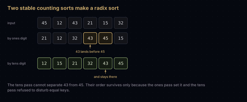
Look at 43 and 45. They share a tens digit, so the second pass cannot tell them apart: both go in the "4" bucket and it has no opinion about their order. The only thing keeping 43 ahead of 45 is that the first pass left them that way and the second refused to disturb equal keys. Stability is not a bonus feature here; it is the mechanism by which earlier passes' work survives.
Break stability and radix sort breaks with it. Here is the same algorithm with one detail changed: the placing pass walks the input backwards while still handing out slots forwards, reversing every group of ties:
def counting_sort_unstable(items: list[Any],
                           key: Callable[[Any], int]) -> list[Any]:
    """The same three phases, but the placing pass runs backwards over the input
    while still handing out slots forwards, which reverses every group of ties."""
    keys = [key(item) for item in items]
    lowest = min(keys)
    counts = [0] * (max(keys) - lowest + 1)
    for value in keys:
        counts[value - lowest] += 1

    starts, running = [0] * len(counts), 0
    for index, count in enumerate(counts):
        starts[index] = running
        running += count

    output: list[Any] = [None] * len(items)
    for item, value in reversed(list(zip(items, keys))):
        slot = value - lowest
        output[starts[slot]] = item
        starts[slot] += 1
    return output


broken_ones = counting_sort_unstable(data, key=lambda value: value % 10)
broken_tens = counting_sort_unstable(broken_ones, key=lambda value: value // 10 % 10)
print(f"by ones  {broken_ones}   (still ordered by last digit)")
print(f"by tens {broken_tens} (not sorted)")by ones [21, 32, 12, 43, 15, 45] (still ordered by last digit)
by tens [15, 12, 21, 32, 45, 43] (not sorted)Each pass is individually correct: check the digits and both outputs are properly ordered by the digit they sorted on. The composition is garbage: 15 before 12, 45 before 43. That is what stability buys, made visible.
Elsewhere
NumPy's stable sort. numpy.sort(kind="stable") maps to a radix sort for small integer types and to Timsort otherwise, and the radix path is counting sort repeated once per byte. Call it on an array of int16 and you have run counting sort.
Suffix array construction. SA-IS, the standard linear-time algorithm for building suffix arrays — the index behind the Burrows-Wheeler transform and many full-text search tools — starts by counting how many suffixes begin with each character and turning those counts into bucket boundaries. Phases 1 and 2, unchanged, before any of the clever induced-sorting work begins.
Image histograms. Histogram equalisation counts how many pixels sit at each of the 256 intensity levels, takes the running total to get the cumulative distribution, then maps every pixel through it. Count, prefix sum, place — counting sort with the last phase repurposed.
GPU sorting. Radix sort is the standard sort on GPUs, and NVIDIA's CUB and Thrust libraries both build it from repeated count-and-scan passes, because both halves parallelise cleanly. A count is a histogram; a prefix sum is a scan, one of the most heavily optimised parallel primitives there is. Comparison sorts have no equivalent structure to exploit.
The standard library gives you phase 1 directly:
from collections import Counter

tally = Counter([2, 5, 3, 0, 2, 3, 0, 3])
print(sorted(tally.items()))
print([value for value in sorted(tally) for _ in range(tally[value])])[(0, 2), (2, 2), (3, 3), (5, 1)]
[0, 0, 2, 2, 3, 3, 3, 5]That second print is a one-line counting sort for bare integers, with a property the array version lacks: it costs O(n + d log d), where d is the number of distinct values rather than the size of the range, so it survives sparse data. It has no phase 2 or 3 at all, so it cannot sort records.
Common mistakes
Sizing the count array with len(values) instead of the key range. These are unrelated numbers. [0] * len(values) on [100, 2, 7] gives three counters and an IndexError on the first value.
Forgetting the + 1. [0] * max(values) leaves no slot for the maximum itself, and the largest value always appears, so at least this one fails loudly.
Assuming non-negative keys. This is the quiet one. Python's negative indexing means counts[-3] += 1 cheerfully increments a counter near the end of the array instead of raising. The tally is wrong, the prefix sums are wrong and the output is wrong, with no exception anywhere. Always subtract the minimum key.
Mixing the two prefix-sum conventions. Exclusive sums pair with a forward scan and an increment; inclusive sums pair with a backward scan and a decrement. Use inclusive sums with a forward scan and every group starts where the next key's block should begin, so each group is displaced into its neighbour's slots and the last one runs off the end of the output.
Losing stability without noticing. An unstable counting sort looks fine in isolation and only fails when composed: inside radix sort, or when someone sorts by a second key expecting the first to survive. Test stability explicitly, with records that have equal keys.
Confusing k with the number of distinct values. Three items valued 1, 5 and 1,000,000 need a million counters. A dictionary of counts avoids the memory on sparse data, but gives up O(1) indexing and the linear-time guarantee with it.
Practice
- Sort a list of lowercase letters by mapping each character to
ord(character) - ord("a")and using a 26-slot count array. - Return the prefix sums alongside the sorted list, and use them to answer "how many items have a key of at most v" in constant time.
- Implement the CLRS variant (inclusive prefix sums, backward scan, decrement), and check it produces output identical to the version above on a list with many ties.
- Write a descending counting sort that still keeps items with equal keys in their input order, and prove it with a list of
(name, score)tuples. - Build LSD radix sort by calling your counting sort once per digit, then sort 1,000 numbers below 1,000,000 with six passes and count the total operations against n log₂ n.
Summary
Counting sort trades generality for speed. It refuses to compare anything, so the O(n log n) decision-tree floor does not apply to it, and it finishes in O(n + k) on every input it is given. What it demands in return is that the keys be integers in a range small enough to allocate an array over, and when that range is large or sparse, the memory cost turns from a footnote into a wall you cannot climb. Its prefix-sum phase is worth learning even if you never call the sort itself, because that step is what makes it stable, and its stability is what makes radix sort possible.
| Difficulty | Medium |
| Best case | O(n + k) — no branch depends on the data |
| Average case | O(n + k) |
| Worst case | O(n + k) — identical to the best case |
| Space | O(n + k) — one counter per possible key, plus an output buffer |
| Stable | Yes — with exclusive starting positions and a forward placing pass |
| In place | No — the output is a separate list |
| Adaptive | No — sorted input costs exactly the same as random input |
| Comparisons | None — every key is used as an array index |
| Data structure | List / array indexed by key value |
| Use it when | Keys are integers over a known range and k is O(n) |
| Avoid it when | k is much larger than n, or keys are floats, strings or unbounded |
| Real-world use | Every pass of LSD radix sort; NumPy's stable integer sort; suffix-array bucketing; image histograms |
| Python equivalent | sorted(items); collections.Counter gives you phase 1 |
The natural next step is radix sort, which takes counting sort's one weakness — that k must stay small — and removes it by chopping large keys into small digits and running a stable counting sort over each one.
Keep reading
- Radix Sort in Python — counting sort applied one digit at a time, and the reason stability matters so much.
- Merge Sort in Python — the comparison sort that sits exactly on the O(n log n) floor described above.
- Big O Notation — why O(n + k) is a sum rather than a product, and what that means in practice.
- Prefix Sums in Python — the running-total trick from phase 2, generalised to range queries.
- Timsort — what
sorted()actually runs, and the sort to beat before writing your own.


