The 0/1 knapsack problem is where dynamic programming stops feeling like a trick and starts feeling like a method. It is also the problem interviewers reach for when they want to know whether you can turn a decision into a recurrence, and a recurrence into a table.
The setup is one sentence. You have a bag that holds a fixed amount of weight, and a pile of items that each have a weight and a value. Take a subset that fits, and make the total value as large as possible. The "0/1" is the whole difficulty: each item is either in the bag or out of it. You cannot take half a laptop, and you cannot take the same laptop twice.
That restriction rules out the obvious approach. Sorting by value per kilogram and grabbing greedily is optimal when items can be cut into pieces, and provably wrong when they cannot. There is a four-item example below where it loses by 10%. What works instead is a table with one row per item and one column per unit of capacity. Everything below builds it: brute force, the recurrence, memoisation, the 2D table, the 1D rolling array, and how to recover which items were chosen. Then the part most write-ups skip: why O(n × W) is not a polynomial bound.
The idea
Line the items up in any fixed order and walk them one at a time. For each item there are exactly two futures:
- Leave it. The capacity is unchanged, and you carry on with the remaining items.
- Take it. The value goes up by that item's value, and the capacity goes down by its weight. You carry on with the remaining items and the smaller capacity.
The best you can do is whichever of those two futures ends up worth more. Written as a function, with best(i, c) meaning "the most value obtainable from items i onwards with c capacity left":
best(i, c) = 0                                   if i is past the last item, or c == 0
           = best(i + 1, c)                      if item i weighs more than c
           = max( best(i + 1, c),                    leave it
                  value[i] + best(i + 1, c - weight[i]) )   take it
That recurrence is correct by construction: it considers both options for every item, so it cannot miss the best subset. It is also the entire algorithm. Everything that follows is bookkeeping to make it fast.
Here is the instance to keep in your head. A courier drone lifts 6 kg, and four parcels are waiting:
| Parcel | Weight | Value | Value per kg |
|---|---|---|---|
| books | 2 kg | 4 | 2.00 |
| tools | 3 kg | 5 | 1.67 |
| paint | 4 kg | 6 | 1.50 |
| tiles | 5 kg | 7 | 1.40 |
Start the recurrence at the first parcel with all 6 kg free, and the calls fan out in a binary tree.
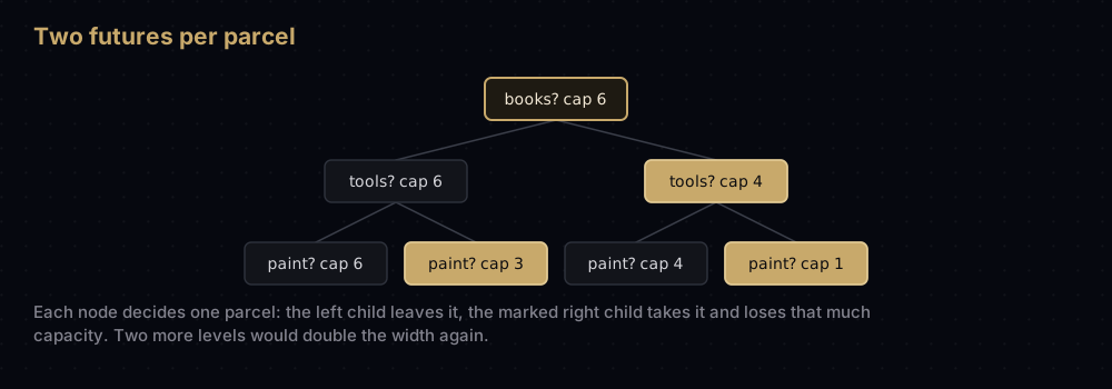
Two things are visible in that tree, and they set up everything else.
The tree doubles at every level. With n parcels the leaves number 2^n, exactly the number of subsets: the recursion is an organised way of trying all of them. Four parcels is 16 subsets, so brute force is fine. Forty parcels is over a trillion, and forty is not a big number of parcels.
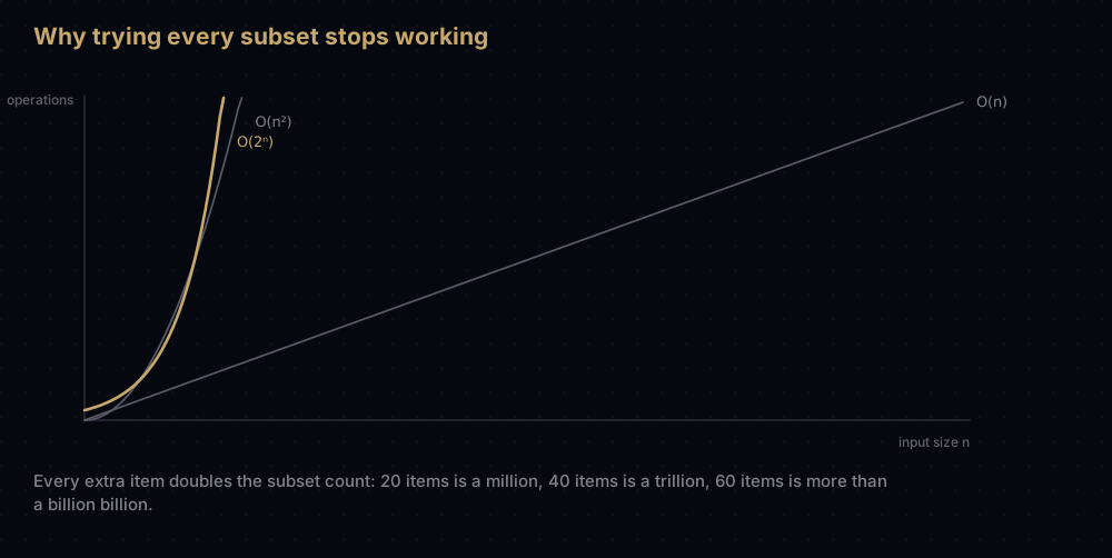
The tree repeats itself. A call is fully described by two numbers: which parcel you are looking at, and how much capacity is left. There are n + 1 values for the first and W + 1 for the second, so however large the tree grows it contains at most (n + 1) × (W + 1) genuinely different calls. Everything beyond that is a repeat. Cache each distinct call and the exponential collapses to a rectangle.
Watching it work
Turn the recurrence around. Instead of starting with all four parcels, start with none and add them one at a time. Build a table where table[i][c] is the best value using only the first i parcels in a bag of capacity c, for every capacity from 0 to 6.
Row 0 — no parcels. Nothing to take, so every capacity is worth 0.
Row 1 — books (2 kg, value 4). Capacities 0 and 1 cannot hold it, so they stay at 0. From capacity 2 upwards, taking books is worth 4 plus row 0's value for the leftover capacity, which is 0. The row is [0, 0, 4, 4, 4, 4, 4].
Row 2 — tools (3 kg, value 5). At capacities 3 and 4, taking tools is worth 5 against 4 for leaving it, so 5 wins. At capacity 5, taking tools is worth 5 plus row 1 at capacity 5 − 3 = 2, which is 4: total 9, books and tools together. Capacity 6 is still 9, because the spare kilogram buys nothing. The row is [0, 0, 4, 5, 5, 9, 9].
Row 3 — paint (4 kg, value 6). At capacity 6, taking paint is worth 6 plus row 2 at capacity 6 − 4 = 2, which is 4: total 10, against 9 for leaving it. The row is [0, 0, 4, 5, 6, 9, 10].
Row 4 (tiles (5 kg, value 7). At capacity 6, taking tiles is worth 7 plus row 3 at capacity 1, which is 0), so 7, against 10 for leaving it. Tiles never make the cut, and row 4 is a copy of row 3.
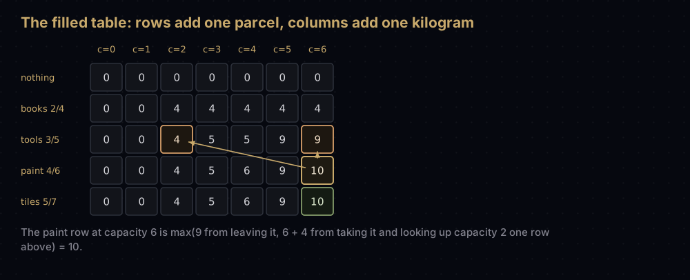
The answer is the bottom-right cell: 10, from books plus paint, weighing exactly 6 kg. Notice what the table did not do: it never sorted anything and never looked at value per kilogram. Greedy ratio order takes books then tools, fills 5 kg, and stops at 9.
Recovering which parcels were chosen
The table holds numbers, not parcels. To find out what to load, walk backwards from the bottom-right corner asking one question per row: is this row's value different from the row above?
table[4][6]is 10 andtable[3][6]is 10. Tiles changed nothing, so tiles were not taken. Move up totable[3][6].table[3][6]is 10 andtable[2][6]is 9. The value rose only because paint was taken, so paint is in the bag. Subtract its 4 kg and move totable[2][2].table[2][2]is 4 andtable[1][2]is 4. Tools were not taken. Move up totable[1][2].table[1][2]is 4 andtable[0][2]is 0. Books were taken. Subtract 2 kg, arrive attable[0][0], stop.
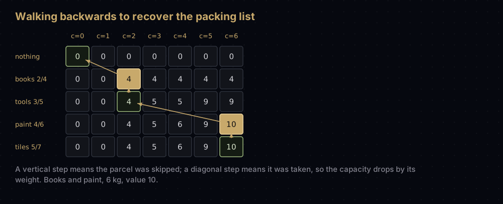
A vertical step means the item was skipped; a diagonal step means it was taken and the capacity dropped by its weight. Four steps for four items: reconstruction costs O(n), not another sweep of the table.
The code
Start with the version that cannot be wrong, so there is something to check the fast versions against.
from typing import NamedTuple


class Item(NamedTuple):
    name: str
    weight: int
    value: int


PARCELS = [
    Item("books", 2, 4),
    Item("tools", 3, 5),
    Item("paint", 4, 6),
    Item("tiles", 5, 7),
]
CAPACITY = 6


def knapsack_brute_force(items: list[Item], capacity: int) -> tuple[int, list[str]]:
    """Try every subset of items and keep the most valuable one that fits."""
    best_value = 0
    best_names: list[str] = []

    # Each bit of `mask` is one item: 1 means in the bag, 0 means left behind.
    for mask in range(1 << len(items)):
        chosen = [item for index, item in enumerate(items) if mask >> index & 1]
        if sum(item.weight for item in chosen) <= capacity:
            value = sum(item.value for item in chosen)
            if value > best_value:
                best_value = value
                best_names = [item.name for item in chosen]

    return best_value, best_names


best, names = knapsack_brute_force(PARCELS, CAPACITY)
print(f"subsets tried: {2 ** len(PARCELS)}")
print(f"best value: {best} by taking {names}")subsets tried: 16
best value: 10 by taking ['books', 'paint']Now the recurrence, transcribed line for line.
def knapsack_recursive(items: list[Item], index: int, capacity: int) -> int:
    """Best value obtainable from items[index:] within `capacity`."""
    if index == len(items) or capacity == 0:
        return 0

    item = items[index]
    leave_it = knapsack_recursive(items, index + 1, capacity)
    if item.weight > capacity:
        return leave_it          # no choice to make, it does not fit

    take_it = item.value + knapsack_recursive(items, index + 1, capacity - item.weight)
    return max(take_it, leave_it)


print(f"capacity 6: {knapsack_recursive(PARCELS, 0, 6)}")
print(f"capacity 4: {knapsack_recursive(PARCELS, 0, 4)}")
print(f"capacity 1: {knapsack_recursive(PARCELS, 0, 1)}")capacity 6: 10
capacity 4: 6
capacity 1: 0Correct, and exponential. Adding a cache is one decorator, and the effect is not subtle. Both versions below count how many times the function body actually executes, on an 18-parcel instance with a 40 kg drone.
from functools import lru_cache

# A deterministic 18-item instance, big enough for the two versions to diverge.
BIG_ITEMS = [
    Item(f"p{index}", index * 7 % 13 + 1, index * 11 % 17 + 1)
    for index in range(18)
]
BIG_CAPACITY = 40


def count_plain(items: list[Item], capacity: int) -> tuple[int, int]:
    """Run the plain recursion, reporting (best value, calls made)."""
    calls = 0

    def solve(index: int, remaining: int) -> int:
        nonlocal calls
        calls += 1
        if index == len(items) or remaining == 0:
            return 0
        item = items[index]
        leave_it = solve(index + 1, remaining)
        if item.weight > remaining:
            return leave_it
        return max(item.value + solve(index + 1, remaining - item.weight), leave_it)

    return solve(0, capacity), calls


def count_memoised(items: list[Item], capacity: int) -> tuple[int, int]:
    """Same recursion, but each (index, remaining) pair is solved only once."""
    calls = 0

    @lru_cache(maxsize=None)
    def solve(index: int, remaining: int) -> int:
        nonlocal calls
        calls += 1
        if index == len(items) or remaining == 0:
            return 0
        item = items[index]
        leave_it = solve(index + 1, remaining)
        if item.weight > remaining:
            return leave_it
        return max(item.value + solve(index + 1, remaining - item.weight), leave_it)

    return solve(0, capacity), calls


plain_value, plain_calls = count_plain(BIG_ITEMS, BIG_CAPACITY)
memo_value, memo_calls = count_memoised(BIG_ITEMS, BIG_CAPACITY)
print(f"plain recursion: value {plain_value} in {plain_calls} calls")
print(f"memoised:        value {memo_value} in {memo_calls} calls")
print(f"distinct states: {len(BIG_ITEMS) + 1} x {BIG_CAPACITY + 1} = "
f"{(len(BIG_ITEMS) + 1) * (BIG_CAPACITY + 1)}")plain recursion: value 100 in 95565 calls
memoised: value 100 in 571 calls
distinct states: 19 x 41 = 779Same answer, 167 times less work, and the memoised count is capped by the 779 possible states: it never reaches the cap because some states are unreachable. lru_cache is the standard-library tool for this and it is genuinely all you need in an interview.
The table version computes the same numbers bottom-up, in a fixed order, with no recursion and no cache lookups.
def knapsack_table(items: list[Item], capacity: int) -> list[list[int]]:
    """Build the full DP table.

    table[i][c] is the best value using only the first i items in a bag
    that holds c units of weight.
    """
    table = [[0] * (capacity + 1) for _ in range(len(items) + 1)]

    for i in range(1, len(items) + 1):
        item = items[i - 1]
        for c in range(capacity + 1):
            leave_it = table[i - 1][c]
            if item.weight > c:
                table[i][c] = leave_it          # it does not fit, no choice
            else:
                take_it = item.value + table[i - 1][c - item.weight]
                table[i][c] = max(take_it, leave_it)

    return table


table = knapsack_table(PARCELS, CAPACITY)
labels = ["nothing"] + [item.name for item in PARCELS]
print(f"{'capacity':>9}  " + "  ".join(f"{c:>2}" for c in range(CAPACITY + 1)))
for label, row in zip(labels, table):
    print(f"{label:>9}  " + "  ".join(f"{value:>2}" for value in row))
print(f"answer: {table[-1][-1]}") capacity 0 1 2 3 4 5 6
nothing 0 0 0 0 0 0 0
books 0 0 4 4 4 4 4
tools 0 0 4 5 5 9 9
paint 0 0 4 5 6 9 10
tiles 0 0 4 5 6 9 10
answer: 10Those are the rows filled by hand above, byte for byte. The backwards walk turns them into a packing list.
def chosen_items(items: list[Item], capacity: int,
                 table: list[list[int]]) -> list[Item]:
    """Walk the finished table backwards to recover which items were taken."""
    picked: list[Item] = []
    c = capacity

    for i in range(len(items), 0, -1):
        # The value changed between rows, so the only way to reach it was
        # to take item i. Otherwise this row simply copied the one above.
        if table[i][c] != table[i - 1][c]:
            item = items[i - 1]
            picked.append(item)
            c -= item.weight

    picked.reverse()
    return picked


packed = chosen_items(PARCELS, CAPACITY, table)
print([item.name for item in packed])
print(f"weight {sum(item.weight for item in packed)} of {CAPACITY}, "
f"value {sum(item.value for item in packed)}")['books', 'paint']
weight 6 of 6, value 10The rolling array
Look at the table code again: row i only ever reads row i - 1. Rows 0 through i - 2 are dead weight. So keep one row, and overwrite it in place.
def knapsack_1d(items: list[Item], capacity: int, trace: bool = False) -> int:
    """0/1 knapsack in O(capacity) space. The capacity loop must count down."""
    best = [0] * (capacity + 1)

    for item in items:
        # Downwards: best[c - item.weight] has not been touched yet this
        # round, so it still holds the previous row's value.
        for c in range(capacity, item.weight - 1, -1):
            best[c] = max(best[c], item.value + best[c - item.weight])
        if trace:
            print(f"after {item.name}: {best}")

    return best[capacity]


print(f"final: {knapsack_1d(PARCELS, CAPACITY, trace=True)}")after books: [0, 0, 4, 4, 4, 4, 4]
after tools: [0, 0, 4, 5, 5, 9, 9]
after paint: [0, 0, 4, 5, 6, 9, 10]
after tiles: [0, 0, 4, 5, 6, 9, 10]
final: 10Four printed rows, and they are the four rows of the 2D table exactly. The whole table is still being computed; it is just never stored.
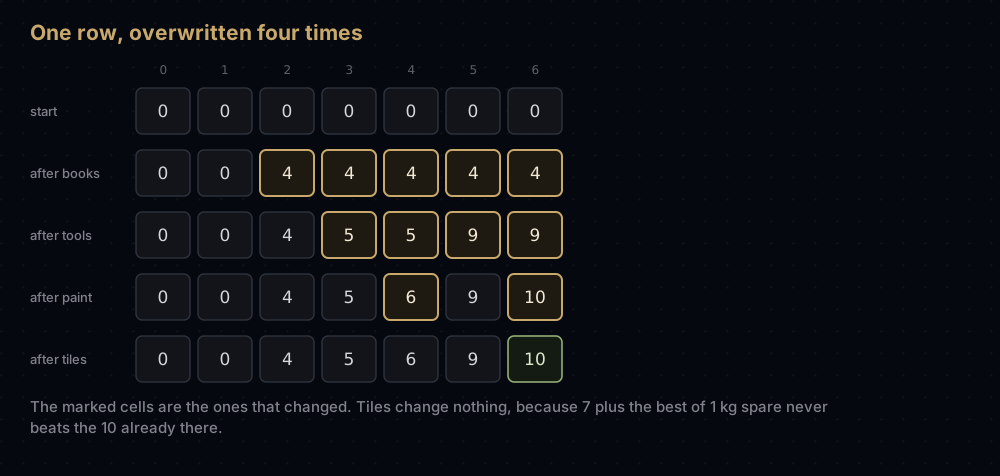
Why the capacity loop must count downwards
This is the one detail that turns a correct solution into a different problem's correct solution, silently. Change range(capacity, item.weight - 1, -1) to range(item.weight, capacity + 1) and everything still runs, still terminates, still returns a plausible number.
def knapsack_1d_upwards(items: list[Item], capacity: int) -> int:
    """The bug: counting upwards turns this into unbounded knapsack."""
    best = [0] * (capacity + 1)

    for item in items:
        for c in range(item.weight, capacity + 1):
            best[c] = max(best[c], item.value + best[c - item.weight])
        print(f"after {item.name}: {best}")

    return best[capacity]


print(f"final: {knapsack_1d_upwards(PARCELS, CAPACITY)}")after books: [0, 0, 4, 4, 8, 8, 12]
after tools: [0, 0, 4, 5, 8, 9, 12]
after paint: [0, 0, 4, 5, 8, 9, 12]
after tiles: [0, 0, 4, 5, 8, 9, 12]
final: 12Look at the first row. Books weighs 2 kg and is worth 4, and the row claims a 6 kg bag is worth 12. That is three copies of books.
Here is the mechanism. The recurrence needs best[c - weight] to mean the previous row: the best you could do without this item. Going upwards, that cell was overwritten a few iterations ago in this same round, so it now means "the best you can do including this item". Adding the item on top of that takes it twice, and the next cell takes it three times.
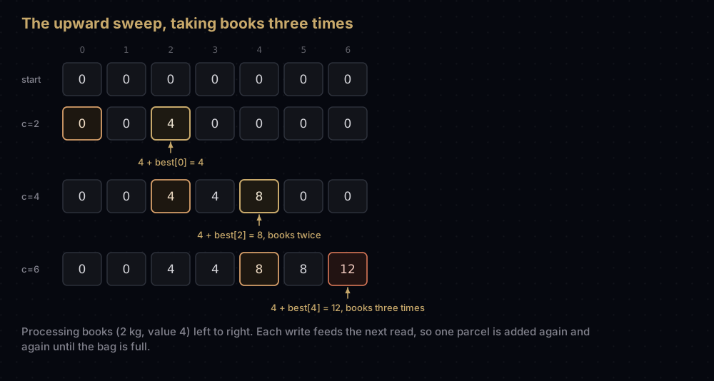
Reads always go leftwards, so a downward sweep only ever reads cells it has not written yet. That is the whole argument, and it is worth being able to say it out loud: read from cells this round has not touched.
The broken version is not useless, though. It is the exact solution to the unbounded knapsack problem, where every item has unlimited supply: 12 really is the best a 6 kg drone can do if the warehouse has endless boxes of books. Two problems, one loop direction apart.
How the code maps to the idea
The + 1 in both dimensions. The table is (n + 1) rows by (W + 1) columns because row 0 means "no items considered yet" and column 0 means "no capacity left". Those are the recurrence's base cases, and having them as real cells is what removes every special case from the inner loop.
The if item.weight > c branch is the "does not fit" line of the recurrence. Without it, table[i - 1][c - item.weight] gets a negative index. Python does not raise on that: it wraps around and reads from the end of the row, so an unrelated capacity supplies a plausible number and the answer is wrong with no traceback. This is the most expensive missing line in a knapsack implementation.
max(take_it, leave_it) is the recurrence's max, and leave_it being table[i - 1][c] is why the table never gets worse as items are added. Every row is greater than or equal to the row above it, cell by cell.
The reconstruction compares rows, not values. table[i][c] != table[i - 1][c] is the only reliable test. If they are equal, some optimal packing skips item i, so take that one. If they differ, every optimal packing of that cell includes item i, because the extra value had to come from somewhere. Preferring the skip on ties is what makes the walk deterministic when several packings tie for best.
Edge cases fall out of the arithmetic. An empty item list gives one row of zeros and returns 0. A capacity of 0 gives a single column of zeros. An item heavier than the whole bag is never taken, because its if branch fires in every column. No guard clauses needed.
The claim that all three implementations agree is worth testing rather than asserting.
import random

random.seed(11)
for _ in range(400):
    count = random.randint(0, 8)
    items = [Item(f"x{k}", random.randint(1, 9), random.randint(1, 20))
             for k in range(count)]
    cap = random.randint(0, 22)

    reference = knapsack_brute_force(items, cap)[0]
    assert knapsack_table(items, cap)[-1][-1] == reference
    assert knapsack_1d(items, cap) == reference

print("400 random instances: brute force, 2D table and 1D array all agree")400 random instances: brute force, 2D table and 1D array all agreeRandom testing against a slow-but-obviously-correct reference is the cheapest way to trust a DP. It catches loop-direction bugs, off-by-ones and missing base cases in seconds.
Complexity
Write n for the number of items and W for the capacity.
Brute force: O(2^n) for the recursion, O(n × 2^n) for the mask loop. Each item doubles the number of subsets, so there are 2^n of them. The recursion builds a binary tree whose leaves are those subsets: fewer than 2^(n+1) nodes, O(1) work each, which is where O(2^n) comes from. On 18 parcels the measured count above was 95,565 calls against the 524,287 nodes of a full depth-18 binary tree; branches that run out of capacity stop early, which prunes some of it and changes nothing about the growth rate. knapsack_brute_force is the more expensive of the two, because it rebuilds and re-sums the chosen list for every mask: that is O(n) per subset, so O(n × 2^n) overall. The extra factor of n is invisible next to 2^n, and it is still the honest bound for the code as written.
The table: O(n × W) time, and that is the best case as much as the worst. The table has exactly (n + 1) × (W + 1) cells, and filling one is a comparison, an addition and two array reads — constant work, no inner loop. The total is (n + 1)(W + 1) constant-cost steps, which is O(n × W). Neither loop bound reads the data, so no input is lucky and there is no early exit: an instance where nothing fits costs exactly what an instance where everything fits costs. The memoised recursion carries the same bound with call overhead on top, and never more, because it only visits states the recursion can actually reach: 571 of the 779 in the run above.
Space: O(n × W) for the table, O(W) for the rolling array. For 1,000 items and a capacity of 100,000, the 2D table is about 100 million Python integers — several hundred megabytes, and probably a swap death. The 1D array is 100,001 integers, well under a megabyte, producing the same answer. The recursive forms carry a cost the loops do not: one stack frame per item, so O(n) of call stack on top of the memo's O(n × W). That is a wall, not a footnote: Python's default recursion limit is 1,000 frames, so the memoised version raises RecursionError somewhere past a thousand items, on an instance the bottom-up table would fill without complaint.
Reconstruction: O(n) time, one step per row, but it needs the 2D table. The rolling array throws away the evidence.
O(n × W) is not polynomial, and this matters
A polynomial-time algorithm is polynomial in the size of its input, measured in bits. The knapsack input is n items plus one capacity number, and writing W down takes about log2(W) bits: a capacity of 1,000,000,000 is 30 bits, not a billion bits. The algorithm still does W units of work per item, so the running time is exponential in the length of the number you typed: add one bit to the capacity and the runtime doubles.
| Capacity | Bits to write it | Cells per item |
|---|---|---|
| 100 | 7 | 101 |
| 10,000 | 14 | 10,001 |
| 1,000,000 | 20 | 1,000,001 |
| 1,000,000,000 | 30 | 1,000,000,001 |
Thirty items with a billion-unit capacity is 30 billion cells, from an input you could write on a napkin. That is a pseudo-polynomial algorithm: polynomial in the numeric value of the input, exponential in its length.
It matters because the decision version of 0/1 knapsack is NP-complete — one of Richard Karp's original 21 problems in 1972 — and this table does not contradict that. Knapsack is only weakly NP-complete: hard when the numbers are large, easy when they are small.
The practical consequence: before writing this table, multiply n by W. A product in the millions is about a second of Python. A product in the billions means this is the wrong tool, however neatly it is written.
When to use it, and when not to
Use the DP when items are indivisible, each is available once, the weights and the capacity are integers, and n × W is small enough to sweep. That covers most interview questions and a lot of genuine scheduling and budgeting work.
Use greedy when the items can be split. In fractional knapsack you may take any fraction of an item, and sorting by value per unit weight then filling from the top is provably optimal. The proof is an exchange argument: if an optimal solution ever includes a unit of a lower-ratio item while a higher-ratio item is still available, swapping that unit raises the total, so no optimal solution can do it. Same instance, both rules:
def fractional_knapsack(items: list[Item], capacity: int) -> float:
    """Greedy by value per unit weight — optimal only when items can be cut."""
    by_density = sorted(items, key=lambda item: item.value / item.weight, reverse=True)
    total = 0.0
    remaining = capacity

    for item in by_density:
        if item.weight <= remaining:
            total += item.value
            remaining -= item.weight
        else:
            total += item.value * remaining / item.weight    # take a slice
            break

    return total


def greedy_whole_items(items: list[Item], capacity: int) -> int:
    """The same greedy rule, but forced to take items whole."""
    by_density = sorted(items, key=lambda item: item.value / item.weight, reverse=True)
    total = 0
    remaining = capacity

    for item in by_density:
        if item.weight <= remaining:
            total += item.value
            remaining -= item.weight

    return total


print(f"fractional greedy: {fractional_knapsack(PARCELS, CAPACITY)}")
print(f"greedy, whole items: {greedy_whole_items(PARCELS, CAPACITY)}")
print(f"dp, whole items: {knapsack_1d(PARCELS, CAPACITY)}")fractional greedy: 10.5
greedy, whole items: 9
dp, whole items: 10Fractional greedy sorts n items and makes one pass, so it is O(n log n) — far cheaper than the table — and it reaches 10.5 by slicing a quarter of the paint. Forced to take whole items, it takes books then tools, fills 5 of the 6 kg and returns 9, which is 10% short. That gap is the entire reason 0/1 knapsack needs dynamic programming; greedy algorithms covers why the exchange argument holds in one case and fails in the other.
Use a different variant when the supply is different. Unlimited copies of each item is unbounded knapsack: same code, capacity loop upwards. At most k copies is bounded knapsack: split each item into copies of size 1, 2, 4, 8, … so that k copies become log2(k) pseudo-items and the 0/1 code runs unchanged. Values equal to weights is subset sum, the same table with booleans.
Avoid the table when the capacity is huge and n is small. For n up to about 40, meet-in-the-middle splits the items in half, enumerates the roughly one million subsets of each half, then sorts one side and binary-searches it: a few tens of millions of operations regardless of how large the capacity is. Avoid it too when weights are real numbers, since scaling 12.75 kg to 1275 multiplies W by 100 and the runtime with it. And avoid it when more than one constraint binds, such as weight and volume and a per-category limit: that is an integer program, and a solver like CBC or HiGHS (reachable from Python through PuLP, OR-Tools or SciPy) will beat any hand-rolled table.
When the values are small but the capacity is enormous, flip the table around: index by value and store the minimum weight needed to reach each value, giving O(n² × maxValue). If an approximate answer is acceptable, scaling the values down before running that table lands provably within any chosen percentage of optimal: a rare case where "99% of the best answer, fast" carries a real guarantee.
Where it shows up in the real world
Capital budgeting. A fixed budget, a list of projects each with a cost and an expected return, each project either funded or not. That is 0/1 knapsack with money as the weight, and it is the textbook operations-research application. The same shape covers grant allocation, marketing spend across indivisible campaigns, and picking which features fit a release with fixed engineering capacity.
Cargo and vehicle loading. A truck, aircraft or container has a hard weight limit and items each worth a known amount to ship. When only weight binds, this is exactly the problem. When volume and axle placement bind too, it becomes an integer program, but the knapsack constraint is still in there.
Inside mixed-integer programming solvers. Any constraint of the form "a weighted sum of 0/1 variables must not exceed a limit" is a knapsack constraint, and solvers such as CBC and Gurobi analyse those constraints to generate cover cuts: extra inequalities that shrink the search space before branching. Knapsack is not only a problem people solve, it is a subroutine inside the tools that solve harder problems.
Cryptography, as a cautionary tale. The Merkle-Hellman knapsack cryptosystem, published in 1978, built a public-key scheme on the hardness of subset sum. Adi Shamir broke it in 1982 by exploiting the "easy" superincreasing knapsack hidden inside the public key. NP-hard in general does not mean hard for the instances you generate.
Common mistakes
Counting the capacity upwards in the 1D version. The headline bug. It compiles, runs, returns a number, and answers a different question, the unbounded knapsack. If your 0/1 answers look too high, check this loop first.
Dropping the if item.weight > c guard. In C this is a segfault or garbage. In Python best[c - weight] with a negative index silently reads from the end of the array, producing a wrong answer that looks reasonable. Either guard the branch or start the loop at item.weight.
Sizing the table n by W instead of n + 1 by W + 1. Without the zero row and zero column you have to special-case the first item and the empty bag, and that is where the off-by-one bugs live.
Reconstructing by re-running greedy over the table. The only correct test is comparing table[i][c] with table[i - 1][c]. Picking "the item that contributes the most" out of the final row does not recover an optimal set.
Assuming the greedy ratio rule is close enough. It is exact for fractional knapsack and can be arbitrarily bad for 0/1. With a 100 kg bag, a 1 kg item worth 2 and a 100 kg item worth 100, greedy takes the higher ratio first — the 1 kg item — and then nothing else fits, for a total of 2 against an optimum of 100. Stretch that gap as far as you like by making the second item heavier.
Treating O(n × W) as polynomial. It is pseudo-polynomial. A capacity given in cents rather than dollars makes the same problem 100 times slower for no extra information.
Practice
- Extend
knapsack_tableso it also returns the total weight actually packed, and confirm it can be below the capacity. - Solve subset sum with the same table: given a list of positive integers and a target, decide whether some subset adds up to exactly the target.
- Write the unbounded version by flipping the capacity loop, then confirm it returns 12 on the four parcels with a 6 kg bag.
- Implement bounded knapsack, where item
ihascount[i]copies, by splitting each item into powers of two and reusing the 0/1 code unchanged. - Count how many distinct subsets achieve the maximum value, rather than just finding one: a second table of counts, filled alongside the first.
Summary
0/1 knapsack is the cleanest example of the dynamic programming method: name the state, write the two-branch recurrence, cache it, flatten the cache into a table, then flatten the table into a single row. The reconstruction walk is the part worth practising, because it turns a number back into a decision. The loop direction is the part worth remembering, because downwards means each item is taken at most once and upwards means it is not.
| Difficulty | Hard |
| Time | O(n × W) in every case — one pass over an n by W table, O(1) per cell |
| Space | O(n × W) for the table, O(W) with the rolling array, plus O(n) of stack if recursive |
| Brute force | O(2^n) recursive nodes — one branch per item; O(n × 2^n) if you enumerate subsets |
| Reconstruction | O(n) — one step per row, needs the 2D table |
| Optimal substructure | Yes — the best for i items is built from the best for i − 1 |
| Greedy works | No for 0/1; yes for fractional knapsack |
| Truly polynomial | No — pseudo-polynomial; W is a value, not an input length |
| Data structure | 2D list of integers, or one rolling 1D list |
| Use it when | Items are indivisible, taken once, weights integral, n × W small enough |
| Avoid it when | Capacity is huge, weights are fractional, or several constraints bind — use a MIP solver |
| Real-world use | Capital budgeting, cargo loading, cover cuts inside MIP solvers |
| Python equivalent | None in the standard library; functools.lru_cache memoises it for free |
Keep reading
- Dynamic Programming Explained — memoisation versus tabulation, and how to spot a DP problem before you have solved it.
- The Coin Change Problem — the unbounded cousin of this table, and another place greedy quietly fails.
- Longest Common Subsequence — a second 2D table with the same backwards reconstruction walk.
- Greedy Algorithms Explained — the exchange argument that makes fractional knapsack optimal and 0/1 knapsack hard.
- Big O Notation — the counting arguments behind O(2^n) and O(n × W).


